what is annotate genome

Write to the Help Desk
Knowledge Articles
NLM Support Center
Knowledge Base

What is genome annotation?

Genome annotation is the process of finding and designating locations of individual genes and other features on raw DNA sequences, called assemblies. Annotation gives meaning to a given sequence and makes it much easier for researchers to view and analyze its contents. To visualize what annotation adds to our understanding of the sequence, you can compare the raw sequence (in FASTA format) with the GenBank or Graphics formats, both of which contain annotations. In both instances note the placement of individual genes and other features on the sequence. When a group of researchers assemble a genome, they may also — with processes they establish themselves — annotate it at the same time. In the past, an assembly with annotation was known as a build . These days, the term build is rarely used, as the genome assembly process and its annotation process are often completely uncoupled. They can be conducted at different times by different parties. For example, the Genome Reference Consortium (GRC) is maintaining and updating the human reference assembly . GRC releases assembly (sequence) updates and deposits these to the International Nucleotide Sequence Database Collaboration (INSDC) without annotation. GRC prepared the latest major assembly update (major release designated as GRCh38) in December 2013 and it has since followed with several minor updates (patches). In further processing of an assembly update, the NCBI staff creates a RefSeq version of the submitted INSDC assembly. Following that, NCBI annotates the RefSeq version of the assembly. Each annotation release has its own designation and time stamp. For example, the latest (as of August 2023) NCBI annotation release is designated as GCF_000001405.40-RS_2023_03 . In addition to the human reference genome, NCBI staff annotate numerous eukaryotic genomes via the powerful Eukaryotic Genome Annotation Pipeline . Visit the Eukaryotic Genome Annotation at NCBI page to start exploring extensive documentation on the annotation process, and to follow the progress of individual genome annotation. NCBI staff have also developed the Prokaryotic Genome Annotation Pipeline that is available as a service to GenBank submitters and also as a stand-alone software package .

An official website of the United States government

The .gov means it’s official. Federal government websites often end in .gov or .mil. Before sharing sensitive information, make sure you’re on a federal government site.

The site is secure. The https:// ensures that you are connecting to the official website and that any information you provide is encrypted and transmitted securely.

Publications
Account settings
My Bibliography
Collections
Citation manager

Save citation to file

Email citation, add to collections.

Create a new collection
Add to an existing collection

Add to My Bibliography

Your saved search, create a file for external citation management software, your rss feed.

Search in PubMed
Search in NLM Catalog
Add to Search

An Introduction to Genome Annotation

Affiliations.

1 Eccles Institute of Human Genetics, University of Utah, Salt Lake City, Utah.
2 USTAR Center for Genetic Discovery, University of Utah, Salt Lake City, Utah.
PMID: 26678385
DOI: 10.1002/0471250953.bi0401s52

Genome projects have evolved from large international undertakings to tractable endeavors for a single lab. Accurate genome annotation is critical for successful genomic, genetic, and molecular biology experiments. These annotations can be generated using a number of approaches and available software tools. This unit describes methods for genome annotation and a number of software tools commonly used in gene annotation.

PubMed Disclaimer

Publication types

Search in MeSH

LinkOut - more resources

Full text sources, miscellaneous.

NCI CPTAC Assay Portal

Citation Manager

NCBI Literature Resources

MeSH PMC Bookshelf Disclaimer

The PubMed wordmark and PubMed logo are registered trademarks of the U.S. Department of Health and Human Services (HHS). Unauthorized use of these marks is strictly prohibited.

Loading metrics

Open Access

Twelve quick steps for genome assembly and annotation in the classroom

* E-mail: [email protected] (HJ); [email protected] (SE)

Affiliations School of Biological Sciences, The University of Queensland, St Lucia, Queensland, Australia, Centre for Agriculture and Bioeconomy, Queensland University of Technology, Brisbane, Queensland, Australia

Affiliation Genecology Research Centre, School of Science and Engineering, University of the Sunshine Coast, Sippy Downs, Queensland, Australia

Affiliation Institute of Marine and Environmental Technology, University of Maryland Center for Environmental Science, Baltimore, Maryland, United States of America

Affiliation Genetics and Breeding Research Center, National Institute of Fisheries Science, Geoje, Korea

Affiliation Biotechnology Research Division, National Institute of Fisheries Science, Busan, Korea

Affiliation Department of Life Science, Chung-Ang University, Seoul, Korea

Hyungtaek Jung,
Tomer Ventura,
J. Sook Chung,
Woo-Jin Kim,
Bo-Hye Nam,
Hee Jeong Kong,
Young-Ok Kim,
Min-Seung Jeon,
Seong-il Eyun

Published: November 12, 2020

https://doi.org/10.1371/journal.pcbi.1008325
Reader Comments

Eukaryotic genome sequencing and de novo assembly, once the exclusive domain of well-funded international consortia, have become increasingly affordable, thus fitting the budgets of individual research groups. Third-generation long-read DNA sequencing technologies are increasingly used, providing extensive genomic toolkits that were once reserved for a few select model organisms. Generating high-quality genome assemblies and annotations for many aquatic species still presents significant challenges due to their large genome sizes, complexity, and high chromosome numbers. Indeed, selecting the most appropriate sequencing and software platforms and annotation pipelines for a new genome project can be daunting because tools often only work in limited contexts. In genomics, generating a high-quality genome assembly/annotation has become an indispensable tool for better understanding the biology of any species. Herein, we state 12 steps to help researchers get started in genome projects by presenting guidelines that are broadly applicable (to any species), sustainable over time, and cover all aspects of genome assembly and annotation projects from start to finish. We review some commonly used approaches, including practical methods to extract high-quality DNA and choices for the best sequencing platforms and library preparations. In addition, we discuss the range of potential bioinformatics pipelines, including structural and functional annotations (e.g., transposable elements and repetitive sequences). This paper also includes information on how to build a wide community for a genome project, the importance of data management, and how to make the data and results Findable, Accessible, Interoperable, and Reusable (FAIR) by submitting them to a public repository and sharing them with the research community.

Citation: Jung H, Ventura T, Chung JS, Kim W-J, Nam B-H, Kong HJ, et al. (2020) Twelve quick steps for genome assembly and annotation in the classroom. PLoS Comput Biol 16(11): e1008325. https://doi.org/10.1371/journal.pcbi.1008325

Editor: Francis Ouellette, University of Toronto, CANADA

Copyright: © 2020 Jung et al. This is an open access article distributed under the terms of the Creative Commons Attribution License , which permits unrestricted use, distribution, and reproduction in any medium, provided the original author and source are credited.

Funding: This work was supported by the Korean Ministry of Agriculture, Food, and Rural Affairs (918010042HD030, Strategic Initiative for Microbiomes in Agriculture and Food) to SE. This work was also supported by a grant from the National Institute of Fisheries Science (R2020001) to WK. The funders had no role in study design, data collection and analysis, decision to publish, or preparation of the manuscript.

Competing interests: The authors have declared that no competing interests exist.

Introduction

Genome projects employ state-of-the-art DNA sequencing, mapping, and computational technologies (including cross-disciplinary experimental designs) to expand our knowledge and understanding of molecular/cellular mechanisms, gene repertoires, genome architecture, and evolution. The revolution in new sequencing technologies and computational developments has allowed researchers to drive advances in genome assembly and annotation to make the process better, faster, and cheaper with key model organisms [ 1 , 2 ].

Such technical advantages and established recommendations and strategies have been widely applied in humans [ 3 – 6 ], terrestrial animals [ 7 – 12 ], and plants and crops [ 13 – 18 ]. Genomic applications in aquatic species that could be potentially important for aquaculture are slower compared with human, livestock, and crops [ 19 – 21 ], compounded by larger diversity, lack of reference genomes, and more novice aquaculture industries. Given that aquaculture is the most rapidly expanding food sector, with the widest diversity of species cultured, it is poised for rapid adoption of genomics applications as these become more accessible. For any specific advice on application of genomics to aquaculture, please refer to previous works [ 19 – 25 ].

Before genome sequencing, a must-have step involves RNA sequencing (RNA-seq) that has provided significant insights into the biological functions [ 26 – 30 ]. RNA-seq plays a key role in genome annotation [ 31 – 36 ] through the identification of protein-coding genes based on transcriptome sequencing data and ab initio or homology-based prediction. However, the use of RNA-seq for genome assembly is limited to genome scaffolding [ 37 ]. While RNA-seq is a powerful technology that will likely remain a key asset in the biologist’s toolkit, recent single-molecule mRNA sequencing approaches (e.g., Pacific Bioscience [PacBio] and Oxford Nanopore Technology [ONT]) have provided significant improvements in gene and genome annotation, making them appealing alternatives or complementary techniques for genome annotation [ 38 – 40 ].

Restriction site–associated DNA sequencing and diversity array technology are cost-effective methods that mainly focus on the detection of loci and the segregation of variants or genome-wide single nucleotide polymorphisms. The generation of genetic linkage maps has been successfully applied to recognize key components in the sustainable production of aquaculture species [ 41 , 42 ]. These attempts have resulted in the emphasis of genomic evaluations/selections or advanced selective breeding programs for desirable traits, such as growth, sex determination, sex markers, and disease resistance [ 42 ]. While these inexpensive techniques have been powerful tools for understanding the genetics of adaptation, recent studies have indicated their limitations for genome scans because they will likely miss many loci under selection, particularly for species with short linkage disequilibrium [ 43 ]. However, the widespread use of whole-genome sequencing (WGS) allows the detection of a full range of common and rare/hidden genetic variants of different types across almost entire genomes.

Many seminal biological discoveries in the 20th century were made using only a genetic analysis of a few selected model organisms because they were readily available for genetic analysis [ 44 ]. However, a high-quality and well-annotated genome assembly is increasingly becoming an essential tool for applied and basic research across many biological disciplines in the 21st century that can turn any organism into a model organism. Thus, securing more complete and accurate reference genomes and annotations before analyzing post-genome studies such as genome-wide association studies, structural variations, and posttranslational studies (methylation or histone modification) has become a cornerstone of modern genomics. Chromosome-level high-quality genomes (including structural and functional annotations) are differentiated from draft genomes by their completeness (low number of gaps and ambiguous N s), low number of assembly errors, and a high percentage of sequences assembled into chromosomes. Advances in next-generation sequencing (NGS) technologies and their analytical tools have made assembling and annotating the genomic sequence of most organisms both more feasible and affordable [ 33 , 45 , 46 ]. Table 1 shows recent chromosome-level genome assemblies and provides a rough estimate of the sequencing depth and costs for beginners to achieve a chromosome-level genome assembly. For diploids, using a minimum 60× depth for PacBio, ONT, 60× for Illumina (San Diego, California, United States of America), and 100× for Hi-C data (Phase Genomics, Seattle, Washington, USA) (an extension of chromosome conformation capture, 3C) is recommended. High-quality end-to-end genome assembly and annotation of small eukaryotic (approximately 1 Gb diploid) and prokaryotic organisms have been achievable with small-to-medium financial resources and limited time, labor, and skill commitments. Nearly all eukaryotic genomes still represent a significant challenge for most aquatic species that have large and complex genomes and no reference genomes.

PPT PowerPoint slide
PNG larger image
TIFF original image

https://doi.org/10.1371/journal.pcbi.1008325.t001

Furthermore, the following fundamental questions should be addressed: Why are genome projects or WGS necessary? What is the aim of a genome project? What kind of information is the research community expected to gather? Even from the beginning of a genome project, describing the expected end product, including project duration/budget, chromosome end-to-end completion, genome browser, and research paper, is required. In particular, if budget is a major obstacle, the best option to raise funds to support the genome project (e.g., industry or government support) must be determined. In addition to the abovementioned limitations, another essential element is bioinformatics, which has become a common denominator to produce and use software that can be applied to biological data in different contexts. As big data and multi-omics analyses are becoming mainstream, computational proficiency and literacy are indispensable skills in a biologist’s toolkit in modern scientific society. All “omics” studies require a certain degree of computational biology: The implementation of analyses requires programming skills and knowledge of computer languages, while experimental design and interpretation require a solid understanding of analytical approaches [ 47 , 48 ]. These could be daunting tasks for biologists who are unfamiliar with computational standards (e.g., codes, pipelines, and system environments) and resources (e.g., SourceForge, Bitbucket, GitLab, and GitHub). While academic cores, commercial services, and collaborations can aid in the implementation of analyses, the computational literacy required to design and interpret omics studies cannot simply be replaced or supplemented [ 47 , 48 ].

In the absence of a standard approach for genome projects, this paper aims to provide practical steps to facilitate project completion before embarking upon a genome assembly and annotation project (mainly for eukaryotic genomes). The target audience is anyone entering this field for the first time, particularly those who do not specialize in genomics research. While we can strive to answer questions in a manner that considers the beginner’s perspective, certain aspects (e.g., assembly algorithms and computer environments) might require further reading for an in-depth understanding.

Step 1: Build a wide community for the project if possible

All genome projects have a common but monumental goal: sequencing the entire target genome for a wide range of genomics applications. While genomics is a rich field, one of the most prominent scientific objectives is probably securing the future of sustainable food sources by harnessing the power of genomics (i.e., desirable traits) [ 19 – 21 , 23 – 25 ], particularly for agriculture. If the species of interest is distinct from the wild, cultured, or harvested, it necessitates networking and building a scientific or stakeholder community to support the project. This usually requires a multi-institutional effort to both initiate and—more importantly—complete the genome project and then interpret the vast quantities of sequencing information produced for any given organism. As expected, WGS/genome projects’ infrastructure demands are particularly high as varying interpretations may require facilities, personnel (skill intensive), and software (knowledge intensive) that suit the needs of immediate analyses, ongoing reanalyses, and the integration of genomic and other phenotype information (or desirable traits). Data storage, maintenance, transfer, and analysis costs will also likely remain substantial and represent an increasing proportion of overall sequencing costs in the future. Moreover, professional groups (including students), expert panels, and field farmers acknowledge that there is a need for educational programs specific to WGS demands. Addressing these needs will likely require substantial investment by agriculture production care systems. Thus, the real cost of WGS—including ongoing maintenance—could be even higher. Despite these burdens, most genome projects bring together leading researchers to work together and build large datasets of DNA from target genomes, which has significantly benefited the research community. These efforts facilitate the sharing of sequence data and help research advance. In particular, smaller research groups that have less experience and are poorly equipped in areas including raw read sequencing and assembly and annotation should consider the main features and steps outlined here via community collaboration. In the case of funding for genome projects, applying for government grants and receiving corporate sponsorships as a consortium could be considered potential solutions as these avenues have been successful for humans, livestock (cow, pig, and sheep), crops (Arabidopsis, rice, and tomato), and aquaculture (salmon, oyster tilapia, and prawn).

Step 2: Gather information about the target genome

Every genome sequencing, assembly, and annotation project is different due to each subject genome’s distinctive properties. There are four fundamental aspects that must be considered when embarking on a new genome project: the genome size, levels of ploidy and heterozygosity, GC content, and complexity. These will directly affect the overall quality and cost of genome sequencing, assembly, and annotation [ 14 , 49 ].

How big is the genome? The genome size will greatly influence the amount of data that must be ordered and analyzed. To assemble a genome, securing a certain number/amount of sequences/depth/coverage (called reads) is the first step before proceeding with ordering sequence data. To get an idea of the size and complexity of a genome, publicly available databases for approximate genome sizes are accessible for fungi ( http://www.zbi.ee/fungal-genomesize ), animals ( http://www.genomesize.com ), and plants ( http://data.kew.org/cvalues ). Selecting a closely related species is a practical option if the information on a target species is unavailable from a public database. Alternatively, the two widely used flow cytometry and k -mer frequency distribution methods could provide reliable genome size estimates to predict repeat content and heterozygosity rates. Flow cytometry is a fast, easy, and accurate system of simultaneous multiparametric analysis for nuclear DNA content including a ploidy level that isolates nuclei stained with a fluorescent dye [ 50 , 51 ]. K -mer frequency distribution, a pseudo-normal/Poisson distribution around the mean coverage in the histogram of k -mer counts, is a powerful and straightforward approach to use raw Illumina DNA shotgun reads to infer genome size, data preprocessing for de Bruijn graph assembly methods (tune runtime parameters for analysis tools), repeat detection, sequencing coverage estimation, measuring sequencing error rates, and heterozygosity [ 52 , 53 ]. It is highly recommended to use both flow cytometry and k -mer methods—the gold standard for genome size measures when designing genomic sequencing projects—because no single sequence-based method performs well for all species, and they all tend to underestimate genome sizes [ 54 ]. Is it a diploid, polyploid, or highly heterozygous hybrid species? If possible, it is better to use a single individual and sequence a haploid, highly inbred diploid organism [ 20 , 23 , 55 ], or isogenic line [ 56 ] because this will essentially minimize potential heterozygosity problems for genome assembly. While most genome assemblers are haploid mode (some diploid-aware mode) to collapse allelic differences into one consensus sequence, using complex polyploid or less inbred diploid genomes can greatly increase the number of present alleles, which will likely result in a more fragmented assembly or create uncertainties about the contigs’ homology [ 14 , 49 ]. If so, polyploid and highly repetitive genomes may require 50% to 100% more sequence data than their diploid counterparts [ 14 ].

Is there high/low GC content in a genomic region? Extremely low or high GC content in a genomic region is particularly known to cause problems for second-generation sequencing (SGS) technologies (also called short-read sequencing: mainly refer to Illumina sequencing), resulting in low or no coverage in those regions [ 57 ]. While this can be compensated for by increasing the coverage, we would recommend using third-generation sequencing (TGS) technologies (PacBio and ONT) that do not exhibit this bias [ 14 , 49 ].

How many repetitive sequences (or transposable elements) will likely be present in the genome? The amount and distribution of repetitive sequences, potentially occurring at different locations in the genome, can hugely influence genome assembly results, simply because reads from these different repeats are very similar and the assemblers’ algorithms cannot distinguish them effectively. This may eventually lead to misassembly and misannotation. This is particularly true for SGS reads and assemblies, and a high repeat content will often lead to a fragmented assembly because the assemblers cannot effectively determine the correct assembly of these regions and simply stop extending the contigs at the border of the repeats [ 58 ]. To resolve the assembly of repeats (or if the subject genome has a high repeat content), using TGS reads that are sufficiently long to include the unique sequences flanking the repeats is an effective strategy [ 14 , 49 ]. Thus, understanding the target genome and generating sufficient sequence data/read coverage is a crucial starting point in a genome assembly and annotation project.

Step 3: Design the best experimental workflow

To meet the experimental goals and answer various biological questions, each application must come with different experimental designs. Above all, the development of high-quality chromosomally assigned reference genomes constitutes a key feature for understanding a species’ genome architecture and is critical for the discovery of the genetic blueprints for biologically significant traits. Once the reference genome has been completed, follow-up post-genome studies can be substantially completed with high accuracy.

While NGS is a useful tool for determining DNA sequences, certain parameters need to be considered prior to running an NGS experiment, such as quality control, SGS versus TGS, read length, read quality/error rate, number of reads, genome read coverage/depth, library preparation, and downstream applications. Recent papers have provided useful recommendations and strategies to ensure the success of NGS experiments by selecting the correct products/technologies and methods for the project [ 14 , 59 – 61 ]. If money is no obstacle, using TGS data (PacBio and ONT) and Hi-C data is recommended [ 14 ], which are also widely accepted approaches for reaching a chromosome-level genome assembly ( Table 1 ) for aquaculture or any other species. While a hybrid approach using Illumina/10x Genomics Chromium (10xGC) and Hi-C data has been proposed as a cost-effective method, this approach’s contiguity could be lower than that of the combination of TGS data and Hi-C data [ 14 ].

Another important point to consider is whether genome assembly should be de novo or reference guided/assisted ( Table 2 ). De novo assembly is the most widely adopted, but when complete genomes of closely related species are available, reference-guided/assisted genome assembly could be an attractive option because of its lower requirements for coverage data and computational memory [ 14 ]. However, early works have warned against its applications in genome assembly because the resultant assemblies may contain biases toward errors and chromosomal rearrangements in the existing reference genome [ 62 – 64 ]. No matter which assembly approaches and technologies are taken, genome assembly’s purpose is to construct a consensus haploid or haploid-phased chromosome-level assembly. Most extensively used genome assemblers typically collapse the 2 sequences into 1 haploid consensus sequence and thus fail to capture the diploid nature of target organisms. While this has been a key challenge in the bioinformatics and biology community, recent works have demonstrated the effectiveness of generating accurate and complete haplotype-resolved assemblies for diploid and polyploid species ( Table 2 ). While we have provided a brief summary of commonly used tools ( Table 2 ), the comprehensive program list focused on TGS reads can be accessed at LRS-DB ( https://long-read-tools.org ). Thus, selecting the appropriate tools and pipelines is important to achieve accurate chromosome-scale assemblies in a timely manner by leveraging speed and sensitivity in the contiguity and quality of genome assemblies.

https://doi.org/10.1371/journal.pcbi.1008325.t002

Step 4: Choose the best sequencing platforms and library preparations

To sequence an organism’s entire genome (WGS), it must be prepared into a sample library from high-quality genomic DNA. A library is a collection of randomly sized DNA fragments that represent the sample input; its size can vary depending on the choice of sequencing technology. Sample library preparation for WGS is dependent on two considerations: (1) the genome size of the target sample organism; and (2) the amount of sample available to be sequenced. Given the vast range of library preparation products, we can only provide general suggestions for library preparations. For more platform-specific library preparation and sequencing guides, refer to the vendor’s products and/or services page. The recommended procedure is to select the best and most cost-effective library preparation and sequencing technology after considering the given research goal and budget.

The rapid adoption of WGS has been facilitated by the development of SGS and TGS technologies, which have dramatically reduced sequencing costs and simplified genome assembly. It is possible to select short (Illumina, 454, SOLiD, and Ion Torrent), long (ONT and PacBio), or a combination (hybrid) read. Comprehensive guidelines (including pros and cons) for selecting the correct sequencing technology have been extensively described in previous works [ 14 , 59 , 61 , 65 ]. Briefly, while SGS technologies can produce high-throughput, fast, cheap, and highly accurate reads of lengths in the range 75 to 700 bp, they show limited ability to resolve complex regions with repetitive or heterozygous sequences, which results in incomplete or heavily fragmented genome assemblies. According to Illumina, widely used SGS technology—the TruSeq PCR-free Library Preparation Kit—is ideal for any size of genome with a large sample input if there is 2 μg of genomic DNA available. However, the Nextera DNA Library Prep Kit (Illumina) is perfect for large and complex genomes with a small sample input. Meanwhile, the TruSeq Nano DNA Library Prep Kit (Illumina) is ideal for any size genome with a small sample input if there is only 200 ng of genomic DNA available. However, the Nextera DNA XT DNA Library Preparation Kit (Illumina) is perfect for small genomes, plasmids, and amplicons. Additional Illumina library preparation methods and sequencing platforms for high throughput have been extensively reviewed [ 66 , 67 ].

Meanwhile, TGS technologies can produce long single-molecule reads (averaging >30 kb) with complete contiguity, facilitating assembly. However, long-read technologies suffer from both high costs per base and high error rates. To overcome this disadvantage, the PacBio RS II or SEQUEL system (Pacific Biosciences, Menlo Park, California, USA) has been released that could generate 10 to 15 times more data than the original SEQUEL system with even more accurate long reads (HiFi reads could be ABI Sanger quality up to 40 kb). According to PacBio, the SMRTbell Template Prep Kit (Pacific Biosciences) with 20 to 40 kb template preparation using BluePippin Size Selection is recommended for WGS [ 14 , 68 ]. For ONT, a combination of ligation sequencing, PCR sequencing, and rapid sequencing has been optimized for WGS [ 60 , 69 ]. In particular, the Rapid Sequencing Kit (SQK-RAD004) could produce even higher read lengths and some reads could be >2 Mb [ 70 ].

Combining data from both SGS and TGS in a “hybrid approach/assembly” can compensate for the downsides of both approaches and is a cost-effective method because SGS data can correct errors in TGS reads [ 33 , 71 – 75 ]. Alternatively, the development of an advanced “hybrid” approach, such as incorporating 10xGC data or medium-size single-molecule DNA fragment selection and tagging before short-read sequencing, could be a practical strategy to increase the continuity and accuracy of long reads [ 14 ]. While recent studies have highlighted the efficacy and cost-effectiveness of 10xGC linked-reads in diploid aquatic species’ genomes [ 76 – 79 ], the utility of this technology for complex and/or polyploid aquatic species is still being investigated. According to 10xGC, the Chromium Genome Reagent Kit is ideal.

Regardless of the sequencing technology and approach (SGS, TGS, or hybrid), incomplete and/or unfinished assemblies can still occur (e.g., those with gaps and fragments). Thus, additional techniques such as optical mapping (BioNano, San Diego, California, USA) and chromatin association (Hi-C) are highly recommended to facilitate contig joining and genome assembly completion [ 46 , 80 – 83 ]. Use of the Hi-C method over BioNano has been observed in aquaculture species ( Table 1 ). The most widely used kit is the Proximo Hi-C Kit provided by Phase Genomics ( https://www.phasegenomics.com/hi-c-kits ).

Step 5: Select the best possible DNA source and DNA extraction method

The extraction of high-quality DNA is the most important aspect of a successful genome project. Given the potential breadth of aquaculture species, each with their own peculiarities, extracted high-molecular-weight DNA should be free of contaminants either from the subjected material itself or from the DNA extraction procedure (e.g., polysaccharides, proteoglycans, proteins, secondary metabolites, polyphenols/polyphenolics, humic acids, carbohydrates, and pigments). While recent publications and commercial kits have provided valuable guidance [ 84 – 86 ], DNA extraction methodologies can be explored and adapted along the lines provided by the literature. In general, the minimum DNA input is required for Illumina and 10xGC > 3 ng, PacBio > 20 μg, ONT > 1 μg, BioNano > 200 ng, and Dovetail > 5 μg [ 14 ]. Depending on the project budget and sequencing platform accessibility, SGS and/or TGS technologies can be considered; we recommend using TGS that can deliver DNA of average size >25 kb. Certain species (e.g., mollusks containing high levels of polysaccharide) warrant more careful planning than others. A modified low-salt cetyltrimethylammonium bromide extraction protocol has produced excellent quality DNA of high molecular weight that is free from contaminants and shearing [ 87 ]. Other important considerations are the heterozygosity rate, amplification, and presence of other tissues/organisms [ 14 , 49 ]. The heterozygosity rate can be reduced using a single individual for extraction. However, certain organisms require a pool of individuals to retrieve a sufficient amount of DNA, which will increase the genetic variability and lead to a more fragmented assembly. Attractive strategies include generating an inbred line of individuals for low-heterozygosity pooled sequencing and/or sequencing of haploid tissues as the foundation for filtering out paralogous sequence variants. These have been successful for cost-effective WGS and for optimizing the precision of allele and haplotype frequency estimates in aquaculture breeding [ 19 , 20 , 24 , 42 , 55 ]. When few cells are available, the genomic DNA must be amplified before sequencing, but this can often result in uneven coverage due to artificial effects (chimeric and/or fused unrelated sequences). The introduction of unwanted/unrelated organisms (e.g., contaminants and/or symbionts) and/or tissues (e.g., mitochondria and/or chloroplasts) should be minimized at the extraction and library preparation stages. This requires using tissue with a higher ratio of nuclear over organelle DNA because this can lead to higher coverage of the nuclear genome in the sequences. Whichever approach is adopted, there will be a need to refine the method to achieve several important quality metrics for genome sequencing.

Care should be taken for quality parameters (e.g., the chemical purity and structural integrity of DNA) and two recent works have made the recommendations outlined below for long-read technologies [ 14 , 49 ]. Generally, the measurement/quantification of purified DNA should be performed using both spectrophotometric and fluorescence-based methods (e.g., qubit). Samples with optical density (OD 260 :OD 280 ) ratios of 1.8 to 2.0 are usually free of protein contamination. DNA concentrations at a 1:1 ratio (determined by spectrophotometry and fluorimetry, respectively) are very good indicators of whether they will be sequenced efficiently. To determine the integrity of DNA samples, contour-clamped homogeneous electric field or pulsed-field gel electrophoresis is appropriate when used with TapeStation or Fragment Analyzer (Agilent Technologies, Santa Clara, California, USA). Analyzing isolated DNA in this manner also facilitates decisions regarding shearing DNA to attain an optimal size range for sequencing. Thus, it is always worth investing time in getting high-quality DNA that will result in high-quality data and assembly to save time and money.

Step 6: Check the computational resources and requirements

Installing open-source tools in one’s computational environment is not always either straightforward or trivial. It generally poses three potential problems: (1) the prerequisites of the tools created by diverse developers employing diverse programming frameworks differ; (2) the installation of various software items in one environment can lead to hard-to-resolve software dependency conflicts; and (3) upon successful installation, maintaining the environment and ensuring that all tools (including changes and updates) are working as expected remain difficult. Therefore, managing the data analysis environment becomes increasingly complex when a project requires many tools for genomic data analysis. While addressing the importance of the appropriate data and computing infrastructure to genome projects is difficult, the two following options (see Step 7: maximizing in-house workers or collaboration and outsourcing from the service provider) can be considered.

Access to high-performance computing or cloud-based computing systems is crucial for genome projects that require a large number of computing resources. As a general guide, the successful assembly of a moderately sized diploid genome (approximately 1 Gb) using software pipelines (Tables 1 and 2 ) requires a minimum computing resource of 96 physical central processing unit (CPU) cores, 1 TB of high-performance random-access memory (RAM), 3 TB of local storage, and 10 TB of shared storage [ 14 ]. However, the guide is scalable based on the amount of data, genome size, heterozygosity rate, and ploidy. Please note that runtimes, memory requirements, number of CPUs, and computational costs will increase geometrically because genome assembly is an all-by-all comparison. However, hard drive space to store raw and/or intermediate data (e.g., storage space) will increase linearly as the total amount/depth of coverage required does not dramatically change as genomes increase in size. In addition, the recommendations stated here will likely apply to larger and more complex genomes (e.g., crustaceans with numerous chromosomes) but at a slower rate and with higher computing resources and costs (obtaining more computing resources will increase costs). If participants’ or collaborators’ institutions are equipped with large in-house high-performance computing resources, they will likely have more direct access and practical assistance in their genome project. Otherwise, cloud-based computing is a potential solution that has been widely emphasized in previous works including easy-to-follow steps [ 88 – 90 ]. While cloud computing provides flexibility, competitive pricing, and continually updated hardware and software, it still requires assistance from information technology (IT) specialists to set up suitable cloud-based software. Thus, users should consider all possible options (including their research budget) to achieve the best outcome.

Step 7: Choose the best computational design and pipeline

Optimizing a computational design and securing sufficient computer resources are essential steps to succeed in a genome assembly and annotation project. In addition, computational proficiency and literacy have become vital skills for biologists to design and interpret big data analyses and multi-omics studies [ 48 ]. Given the vast range of computational tools and requirements (different resource demands between assembly and annotation for each species), general suggestions are provided on the computational aspect. However, when establishing the best and most cost-effective computational design and requirement, it is important to consider three options: (1) maximizing in-house workers or collaboration; (2) outsourcing from a service provider; and (3) simulating data with different settings. Ultimately, the most suitable and practical approach in methodological computational biology research is recommended because there is no perfect computational design for genome assembly and annotation.

Before embarking on any actual data analyses, the overall goals should first be defined by understanding in-house workers and facilities because computational design requires extensive learning of computer and biology knowledge, which is a great challenge for most wet lab researchers/groups. If in-house workers and computer facilities are not ready to deliver successful outcomes, cross-disciplinary collaborations (computer science, data science, bioinformatics, and biology) could present great solutions. Initiating and successfully maintaining cross-disciplinary collaborations can be challenging but are highly rewarding because the combination of methods, data, and interdisciplinary expertise can achieve more than the sum of the individual parts alone [ 91 ].

Alternatively, work can be outsourced to a service provider. Outsourcing has the following benefits: (1) no need to hire more employees for computational design and analysis, which will reduce labor costs; and (2) there are more talents available at well-equipped companies that are very specialized in specific research fields. However, outsourcing also has the following disadvantages: (1) a lack of control as a contractor; (2) limited methods of communication (e.g., phone, e-mail, or online chat); and (3) the potential danger of poor quality work due to the inability to optimize pipelines (e.g., parameters) and outcomes.

No matter which approach is taken, the essential part is to have firsthand experience to select proper computational design and pipeline and to accurately interpret analyzed genome data. Due to its extensive range of analytical tools and application areas, employing an effective simulator (from the quality of raw reads to assembly evaluation) has become an essential step for benchmarking genomic and bioinformatics analyses [ 92 – 94 ]. In simulations, considering a (very) large number of datasets is generally not a problem, except when the analysis of each dataset is hugely computationally expensive (e.g., in the genome assembly stage). In practice, one should generate and analyze as many datasets as computationally feasible before embracing real empirical studies, particularly before undertaking real assemblies. In large genome assembly, simulating assemblies of down-sampled real data (e.g., 30× coverage/depth of genome) would be very useful for selecting the best pipeline and parameters without requiring too much computational time or cost. Ultimately, a simulation’s practical relevance depends on the similarity between the considered simulation settings and the real datasets in the area of application. The new method may be assessed in different ways depending on the context (e.g., by conducting simulations, applying the method to several real datasets, applying flexible parameter settings, and checking the underlying assumptions in practical examples). Therefore, simulations should not be limited to artificial datasets that correspond exactly to the assumptions underlying the new method as this would favor the new method [ 61 , 95 – 98 ].

Step 8: Assemble the genome

Regardless of which pathway/strategy is chosen, the TGS approach is recommended over the SGS or hybrid approaches. In general, using multiple programs at each stage to predict the best assembly and annotation ( Table 2 ) is also recommended because each approach and tool has limitations based on the problems inherent in the different algorithms and assumptions used. If the abovementioned steps (Steps 1–7) are met, the recommended flowchart and/or guideline for genome assembly, annotation, maintenance, and community effort would be as shown in Fig 1 , which could be broadly applicable to any species. The rationale of each computational design, workflow, and decision tree is well described in Jung and colleagues [ 14 ], including the background information for each of their steps and the spectrum of available analytical options. Following the workflow and decision tree described by Jung and colleagues, the recommended tools herein are the TGS pipeline: PacBio/ONT read sequencing (remove all contaminated DNA; plastids/bacterial contamination) → read quality assessment, evaluation, and filtering → assembly → error correction and polishing using SGS reads → assessment → chromosome-level assembly using BioNano and Hi-C data. Several recent assemblies adopted from this pipeline (or similar) have shown notable improvements in the assembly of intergenic spaces and centromeres [ 33 , 72 ]. A potential assembly outcome from the new SEQUEL II (HiFi) reads would be even more promising (see Step 4) compared to its early version SEQUEL. In the SGS pipeline, if the target is a diploid organism, starting from 10xGC read sequencing over Illumina reads is ideal. Based on the results of the hybrid-based assemblies, the recommended pipeline starts from PacBio/ONT, and 10xGC read sequencing greatly helps build a highly accurate contiguous genome [ 78 ]. However, all assembly approaches/designs derived only from sequence reads will still contain misassemblies (inversions and translocations), these are mainly caused by the inability of both sequencing and assembly pipelines to cope with long tracts of repeat sequences or high levels of heterozygosity and polyploidization. Thus, using BioNano and Hi-C data is highly recommended for reaching chromosome-level assembly because these two methodologies/technologies can improve the assembly quality by validating the integrity of the initial assembly, correcting misorientations, and ordering the scaffolds.

NGS, next-generation sequencing.

https://doi.org/10.1371/journal.pcbi.1008325.g001

Step 9: Check the assembly quality before annotation

In the shotgun sequencing era, assembling a new genome mostly relies on computational algorithms and experimental designs (see Steps 6 and 7). The performance of such algorithms and designs, read lengths, insertion size of sequencing libraries, read accuracy, and genome complexity determines the accuracy and continuity of the genome assembly. Therefore, while estimating assembly quality is an unpredictable and challenging task that requires several statistical and biological validations, it remains an important step for a high-quality genome. Typically, the quality assessment for draft assemblies is carried out via statistical measurements and alignment to a reference genome (if available) [ 99 ]. These include overall assembly size (determining the match to the estimated genome size), measures of assembly contiguity (N50, NG50, NA50, or NGA50; the number of contigs; contig length; and contig mean length), assembly likelihood scores (calculated by aligning reads against each candidate assembly), and the completeness of the genome assembly (Benchmarking Universal Single-Copy Orthologs [BUSCO] scores and/or RNA-seq mapping) [ 100 , 101 ]. In computational biology, N50 is a widely used metric for assessing an assembly’s contiguity, which is defined by the length of the shortest contig for which longer and equal-length contigs cover at least 50% of the assembly. NG50 resembles N50 except for the metric, which relates to the genome size rather than the assembly size. NA50 and NGA50 are analogous to N50 and NG50 where the contigs are replaced by blocks aligned to the reference [ 99 ]. Thankfully, recent bioinformatics tools offer an automated pipeline to compute and evaluate the new genome quickly and accurately in a practical setting [ 44 , 102 , 103 ].

Additional strong indicators of quality include agreement with data on quantitative trait loci, expressed sequence tags (ESTs), fluorescent in situ hybridization experiments employing bacterial artificial chromosome clones, and the genome assembly’s contiguity with a chromosome-level genetic map. If the initial assembly attempt is unsatisfactory, three specific areas (contiguity, accuracy, and completeness) should be considered to determine the best path forward to improve the new assembly’s quality [ 14 ]. Generally, the best way to address high contig numbers with low average size is to acquire and incorporate more TGS or 10xGC (see Steps 3 and 4: hybrid assembly approaches) reads. When attempting to increase assembly quality, adding more and longer TGS reads tends to be more helpful for bridging existing contigs by increasing the size of the average contig; then, subsequently adding further BioNano and Hi-C data improves read accuracy and assemblies’ overall contiguity. Unfortunately, additional BioNano and Hi-C data without TGS reads are unlikely to help increase the assembly quality because the data are usually ineffective at assisting hybrid assemblers span gaps between existing contigs [ 14 ]. To obtain a complete genome, applying LR_Gapcloser, a fast and memory-efficient approach using long reads, would be an excellent choice to close gaps and improve the contiguity of genome assemblies [ 104 ].

Step 10: Genome annotation

Unlike advanced and revolutionized genome sequencing and assembly, getting genome annotation correct remains a challenge. Annotation is the process of identifying and describing regions of biological interest within a genome (both functionally and structurally). While there are various online annotation servers ( Table 3 ), the intended use of the curated data needs to be clearly defined after considering the two options addressed in Step 7 (maximizing in-house workers/collaboration and outsourcing) because the gene-finding problem in eukaryotes is far more difficult than that in prokaryotes such as bacteria. This procedure requires advanced bioinformatics skills, pipelines, and computing resources and consists of three main steps: (1) identifying noncoding regions; (2) identifying coding regions (called gene prediction); and (3) attaching the biological information of these elements.

https://doi.org/10.1371/journal.pcbi.1008325.t003

Recent works have described genome annotations well [ 13 , 105 – 109 ]. However, it is highly recommended that beginners select automatic or semiautomatic annotation methods (including the workflow and guideline in Fig 1 ) because manual annotation can be very time- and labor-intensive and expensive. Note that while automatic procedures help accelerate the annotation process, they decrease the confidence and reliability of the outcomes because results from different servers and/or databases are often dissimilar [ 106 , 110 , 111 ]. Furthermore, automatic annotation algorithms, frequently based on orthologs from distantly related model organisms, cannot yet correctly identify all genes within a genome and manual annotation is often necessary to obtain accurate gene models and gene sets [ 106 , 110 , 111 ]. Thus, a scheme to obtain consensus annotations by integrating different results, a semiautomatic method, is in demand because this could balance automatic and manual approaches, which would increase the reliability of the annotation while accelerating the process [ 106 , 110 , 111 ]. In general, the identification of noncoding regions includes small and long sequences including repetitive and transposable elements ( Fig 1 and Table 3 ). Despite an explosion of interest in noncoding data and the massive volume of scientific data, selecting the best strategy to annotate and characterize noncoding RNAs is a daunting task because of the strengths and weaknesses of each computational and empirical approach [ 112 ]. After screening noncoding regions (e.g., repeat masking and transposable elements), elements of the gene structure (e.g., introns, exons, coding sequences [CDSs], and start and end coordinates) can be predicted for coding regions.

Both ab initio and evidence-based prediction approaches are widely used as each approach has pros and cons. While Augustus and SNAP are the most popular tools for ab initio prediction, they still necessitate the information of the closely related gene and genome model for screening against the newly sequenced genome. By contrast, evidence-based prediction usually uses results obtained by aligning ESTs, protein sequences, and RNA-seq data (results are even better with full-length Iso-Seq data from PacBio or ONT) to a genome assembly as external evidence. Trained gene predictors (training with Augustus and SNAP to obtain more accurate annotation results is highly recommended) can be used in MAKER, BRAKER, and StringTie ( Fig 1 and Table 3 ). When extrinsic evidence from RNA-seq and protein homology information is available, any program/pipeline could be useful for the de novo annotation of novel genomes. In particular, if any RNA-seq data and a genome sequence are available, starting from MAKER and BRAKER over StringTie would be a better choice for a first-time user because MAKER and BRAKER include ab initio prediction (e.g., Augustus training) unlike StringTie (evidence-based prediction only). However, MAKER could be a better choice for updating existing annotations to reflect new evidence. If various gene prediction methods and tools are used to derive the gene structure from a genome, combining these results to obtain the single consensus gene structure via Evidence Modeler, GLEAN, Evigan, or GAAP is essential ( Table 3 ). In particular, BRAKER, StringTie, PASA, and GAAP can update any gene structure annotation by correcting exon boundaries and adding untranslated regions and alternatively spliced models based on assembled transcriptomic data. The evolutionary rapid emergence of new genes (which quickly respond to changing selection pressures) could give rise to orphan genes that might share no sequence homology to genes in closely related genomes [ 113 ]. Combining the methods and results (especially MAKER, BRAKER and StringTie) could therefore prove effective in increasing the number and accuracy of annotation predictions assigned to orphan and any other young genes.

Subsequently, functional annotation—the process of attaching biological information to gene or protein sequences—must be performed. This can be carried out through homology search and gene ontology (GO) term mapping. To investigate gene function or predict evolutionary associations, newly assembled sequences should be compared with gene sequences with known functions to find sequences with high homology using BLAST, Cufflinks, TopHat, GSNAP, Blast2GO/OmicsBox (referred to here as Blast2GO), and GAAP ( Fig 1 and Table 3 ). To label more diverse biological information, GO term mapping should be performed, which allows information about gene-related terms and relations between genes to be stored in three categories: biological processes, molecular functions, and cellular components. Mapping is the process of retrieving GO terms associated with hits (mapping sequences) obtained via a previous homology search (mainly BLAST) that are accessible from AmiGO, Blast2GO, GO-FEAT, and eggNOG-Mapper. Starting from Blast2GO would be a practical choice for a complete novice because it has more graphic user interface mode with explanations.

While Fig 1 and Table 3 provide a summary of useful tools with key features, it is highly recommended to be familiar with the regular update of public databases and pipelines. In addition, understanding the performance and capability of various analysis from a detailed comparison and instructions of common features of annotation tools could be a very important factor for a successful genome annotation, structurally [ 7 , 111 , 114 – 117 ] and functionally [ 8 , 118 – 123 ].

Step 11: Build a searchable and sharable output format

Research papers and data products (researchers are usually required to submit raw sequencing data to appropriate repositories such as Sequence Read Archive [SRA]) are key outcomes of the scientific enterprise, including most successful genome projects. In addition, most genomic projects/data potentially have value beyond their initial purpose but only if shared with the scientific community, including refining assembly and annotation (see Step 12). In recent years, genomic studies have involved complex datasets such that biologists have become “big data practitioners” [ 124 ] because of improvements in high-throughput DNA sequencing and cost reductions. As a result, genomic studies have become routine procedures, and there is widespread demand for tools that can assist in the deliberative analytical review of genomic information. What happens to the data after such projects end? In general, data or data management plans have become the central currency of science because open access, open data, and software are critical for advancing science and enabling collaboration across multiple institutions and throughout the world and increasing public awareness [ 125 ]. For example, when archiving sequencing data, repositories such as those run by the National Center for Biotechnology Information (NCBI) and European Bioinformatics Institute (EBI) both provide locations for data archiving and encourage a set of practices related to consistent data formatting and the inclusion of appropriate metadata. However, this is a difficult task for an individual research group due to the wide variety of data formats, dataset sizes, data complexity, data use cases, ethical questions, and data collection/storage/sharing practices [ 124 , 126 – 128 ]. Despite its importance, major barriers remain to sharing data, software, and research products throughout the scientific community because of the difficulties that interdisciplinary and/or translational researchers face when engaging in collaborative research [ 124 , 125 , 127 ]. To this end, recent works have provided principles that can be applied in genomic data/database projects, including data sharing and archiving via collaborations [ 124 – 128 ].

The following three fundamental questions on this topic should be considered: (1) Do you want to share your data? (2) Do you have enough in-house expertise and infrastructure to maintain and improve the data, including data storage space? (3) Do you want to form internal and external collaborations to increase research productivity? While each research group has different experiences and criteria in collaborations that included data sharing, engaging with multisite collaborations is highly recommended to overcome more pitfalls, including open-ended questions/concerns on genomic data. In addition, sharing open genomic data can easily facilitate reproducibility and repeatability by reusing the same genomic data.

Step 12: Reach out to the community to refine the assembly and annotation

Dropping whole-genome shotgun sequencing costs and improvements in bioinformatics pipelines and computer capabilities have resulted in the situation where a small lab can undertake genome projects (assembly and annotation), and any organism can become a model species. Ironically, the ease of sequencing and assembly presents another challenge for annotation: contamination of the assembly itself, because errors in assembly can cause errors in the annotation (structural and functional). In addition, it is important to ensure that methods are computationally repeatable and reproducible because there have been numerous reports of instability arising from a mere change of Linux platform, even when using the exact same versions of genomic analysis tools [ 49 ]. When including new data, it is also necessary to provide software infrastructure to assist in genomic data updating. Hence, assembled genomes and curated annotations should not and cannot be considered perfect, static, or “final products.” Data must be maintained, refreshed, and updated to ensure their reuse and discovery.

Manual and continuous annotation is critical to achieving reliable gene models and elements; however, this process can be daunting and cost prohibitive for small research communities. While some genome consortia choose to manually review and edit sets via time- and resource-intensive meetings that often require substantial expertise, this still provides opportunities for community building, education, and training. In contrast, for small research groups, it has been proposed that involving undergraduates in community genome annotation consortiums can be mutually beneficial for both education and genomic resources [ 106 ]. Alternatively, a collaborative approach using web portals such as Apollo, JBrowse, G-OnRamp (Galaxy-based platform), and ORCAE [ 129 – 133 ] could be sufficiently robust and flexible to enable the members of a group to work simultaneously or at different times to improve the biological accuracy of annotation.

Despite any community-based participatory research approaches taken, the recruitment and coordination of researchers are central to any research project due to the requirement of diverse expertise and collective learning. The ideal way would be to form a national/international collaborative research partnership with diverse organizations [ 19 , 134 – 136 ]. Alternatively, active promotion via social networks and/or web portal setup could be the most effective way (e.g., Twitter, the Ensemble website, and blogs). Finally, build collective research solidarity by attending conferences would be plausible. There have been previous successful community efforts and involvement in plant ( https://nbenth.com/annotator/index , https://solgenomics.net , and https://www.helmholtz-muenchen.de/pgsb ) and animal genome projects ( http://www.slimsuite.unsw.edu.au/servers/apollo.php , https://bovinegenome.elsiklab.missouri.edu , http://www.gmgi.org/genomics-fish-shellfish , and https://www.sanger.ac.uk/science/data/vertebrate-genomes-sequencing ) using the Apollo instance with J Browsers exhibits attractive and effective routes because it is always online, curators can log in whenever they have time, and some minor revisions only require a few seconds (to confirm the gene models). Others require up to 20 minutes to change (UTR boundaries and other structural alterations).

After the initial setup, tasks include maintaining momentum and morale, according to the recommendations described by Pedro and colleagues [ 137 ]. Participants bring their own experiences and strengths into this effort. Availability of a training webinar (e.g., https://bit.ly/3gauwn7 and https://bit.ly/36iNQds ) would greatly help kick-start the process, alongside a clear set of starting tasks (e.g., a list of genes/families or regions assigned to each curator) and engagement by the community leader. The leader—an enthusiastic champion—can (1) drum up support from their collaborators; (2) fuse community expertise with resources; (3) oversee the project; and (4) act as a liaison between new members wanting to join, the infrastructure provider, and existing annotators. Considering that the collective expertise within a group may be extensive but diverse, it is necessary to standardize the curation for quality control of annotations. To minimize any conflicts that may arise during the annotation process, it is important (1) to have the initial training webinar by laying out clear rules and guidelines; (2) to select a small subset of genes and ask a group of experienced curators to evaluate whether the decisions taken in each case were uniform and sensible; (3) to record webinar training and comments regarding consensus or disagreements for reporting back to the curation team and to edit the tutorial and guidelines; (4) to address this by automated checks and controls (Apollo does not allow this for now or makes it extremely difficult); and (5) to ask multiple reviewers to check each region by reviewing the annotation history in Apollo (labor-intensive method).

Pooling the expertise, resources, and time of active communities could enable a wide range of geographically distance members to participate in a common process, to share and validate the identification of contradictions and the misrepresentation of data on the genomes [ 137 ]. After corrections, the datasets (manually verified gene sets) that emerge from these projects can be used to improve the gene sets for closely related genomes and downstream analysis. Dialog and collaboration between community members have an enormous impact. The result of an entire community agreeing on and taking ownership of a single gene set is a major stepping-stone to accelerating the field. Handling the mammoth task of manual gene annotation in the absence of dedicated funding or teams is a great challenge. However, our guidelines could provide a manageable solution for the prospect of this approach becoming commonplace and will continue to engage in community-driven curation efforts.

Advice for new genomic users to select a basic assembly and annotation pipeline

For a complete novice, our recommendation would be as below (not recommended starting from Illumina only short reads assembly).

Pure long-read assembly: PacBio or ONT read sequencing (if combined, PacBio 40X and ONT 25X, or 60X for a single platform) → CANU assembler (alternatively Flye) → BUSCO assessment → Make a decision to add more sequencing data or proceed next step (See Confirm and Refine in Fig 1 ) → Optional BioNano with RefAligner (still expensive compared to Hi-C data) → Hi-C with 3D-DNA (alternatively HiRise or AllHiC) → Gapclosing with LR_Gapcloser → Arrow with long-read (alternatively Racon) or Pilon polisher with short-read → BUSCO assessment.
Hybrid assembly: 10xGC read with Supernova → PacBio or ONT read with CANU (alternatively MaSuRCA) → The rest are same with “Pure-read assembly” from BUSCO assessment to BUSCO assessment.
Annotation: NCBI or EBI (a web-based automatic pipeline) → If not, proceed a semiautomatic pipeline starting from structural annotation → RepeatMasker → Ab initio Augustus training with MAKER (alternatively BRAKER) → Evidence-based prediction (RNA-seq) with MAKER (alternatively BRAKER) → Noncoding RNA prediction with NONCODE → Functional annotation with Blast2GO (alternatively AmiGO) → Genome Browser.

Conclusions

There are no gold standards for genome assembly and annotation. However, the availability of NGS data (particularly TGS data) and their analytical tools has enabled the sequencing of several high-quality genomes of species of importance in aquaculture in recent years. Beginners and small research groups still face challenges, because genome assembly and annotation are usually complex analytical procedures (or pipelines) requiring interdisciplinary collaborations (from biology to computer science) and hefty costs for refining/maintaining the genome. The recommendations addressed here are broad guidelines that could be considered to avoid common pitfalls throughout the whole-genome assembly and annotation process. However, the comprehensive features (e.g., advantages and disadvantages) of each step and/or technology have not been extensively discussed.

Finally, newly emerging technologies and analytical tools could dramatically improve end-to-end genome assemblies and annotations in the future by replacing the years-long efforts of the past with rapid and low-cost solutions. Meanwhile, emphasis should be placed upon the following: First, define the achievable research aim. Second, avoid the trap of trying to secure a perfect/complete genome assembly and annotation, which could lead to a never-ending project. Third, perform assembly and annotation to gain firsthand experience, including in bioinformatics. Fourth, seek internal and external help and advice from experts. Lastly, be open to sharing genomic data to both increase research productivity and promote public awareness.

Acknowledgments

The authors are grateful to their colleagues, collaborators, and field/technical specialists from each company for their valuable comments.

View Article
PubMed/NCBI
Google Scholar
116. König S, Romoth L, Stanke M. Comparative Genome Annotation. In: Setubal JC, Stoye J, Stadler PF, editors. Comparative Genomics: Methods and Protocols. New York, NY: Springer New York; 2018. pp. 189–212.

Annotation guidelines

Introduction.

This introduction is inspired by the manual curation guidelines from the pea aphid genome, from Stephen Richards (Baylor College of Medicine) and Legeai et al. Insect Mol Biol 2010

A high quality genome sequence is a prerequisite for whole genome analyses but further, robust and complete annotations are essential for a genome to be fully utilized by the scientiﬁc community. Genome annotation involves mapping features such as protein coding genes and their multiple mRNAs, pseudogenes, transposons, repeats, non-coding RNAs, SNPs as well as regions of similarity to other genomes onto the genomic scaffolds. Many of these features can be automatically predicted by sophisticated software packages based on sequence or structure comparisons.

Beyond this point, it is the goal and the job of a community annotation to generate accurate lists of the most crucial and interesting genes from a new genome, with raw data in the form of gene predictions with numbers attached, gaps in the draft genome sequence, and transcriptome alignments. In short, the goal at this point, is to convert the raw, machine generated data into a useable and useful data resource that will advance research in new, powerful and exciting directions.

Some goals of manual annotation are:

To establish almost exhaustive lists of genes playing a key role in some crucial process
To look at your genes of interest enough to be comfortable that you have the right one’s before writing a paper.
To provide names for the known genes – based primarily on homology to what is known in other organisms.
To fix obvious errors in the automated gene models and improve them where additional data is available – i.e. to get the intron/exon co-ordinates right.

For all of the steps, we decided to use Apollo because it offers many functionalities facilitating the correction of gene structures and allowing users to probe, manipulate and alter the interpretation of gene models. Within Apollo, annotations can be created, deleted, merged, split, classiﬁed and commented on. For example, one can easily locate and correct incorrect splice sites or start/stop codons, classify a gene as a pseudogene, and even create a new alternatively spliced RNA.

Accessing the genome homepage

Each genome hosted on BIPAA have a dedicated home page, accessible from AphidBase , ParWaspDB or LepidoDB . Depending on the genome, the access can be restricted to members of the genome sequencing/annotation project. In this case, you will need to login with your BIPAA account that you must create on https://bipaa.genouest.org/account .

From the genome homepage, you get access to different web applications to explore and annotate the genome.

On this page there are 3 important elements

At the bottom, a list of officially released data associated to this genome: usually an assembly, an automatic annotation (or OGS for Official Gene Set), and corresponding functional annotation (InterProScan, Blast vs NR, Blast2GO)
In the middle, a search field allowing to search for you favorite gene based on its ID, or it’s functional annotation (e.g. type “gustatory receptor” to find all genes having a similarity with a known gustatory receptor)
At the top of the page, a menu giving access to all the web applications you will need to manually annotate this genome: a Blast form, a genome browser (JBrowser), Apollo. You can also download the officially released data from the “Download” link in this menu.

For a brief introduction on the available resources for each genome, look at these introduction slides .

Overview of the annotation process

At the beginning of the annotation project, an assembly and an OGS (Official Gene Set) are officially released.

The OGS is the result of an automatic annotation usually performed using the Maker pipeline . Various data is used by Maker to generate this annotation, including RNASeq mapping data, alignments of transcripts and proteins from related species, masking of Repeated Elements.

Once released, the manual curation process can begin. Using Apollo, annotators are invited to manually check that their genes of interests were correctly predicted by Maker. When needed, modifications can be made to the structure of each gene. Finally, a minimum set of information must be associated to each manually curated gene: name, symbol, GO terms (Gene Ontology terms), …

To avoid mistakes, a personal report is generated each night for each annotators, giving access to the list of annotated genes, and the possible corresponding errors and warnings (missing symbol, wrong name, …).

Regularly, a new OGS is released: it is the result of merging the original OGS with the manual curation performed by annotators. When a manually curated gene is in the same location as a gene originally predicted by Maker, it is the first one that is kept, replacing the second. Gene ids are conserved between each OGS release, a suffix being incremented when a gene is modified (structure or associated information like name or symbol).

Each OGS will appear on the genome Homepage shortly after its release.

Using Apollo

Apollo allows to collaboratively improve the genome annotation, both by correcting gene structures and by adding information on gene models.

A curation introduction and a detailed tutorial on how to use Apollo are available here (thanks to Monica Munoz-Torres !):

Detailed examples are available in these slides (thanks to Robert Waterhouse !).

You can also have a look at video recordings of these slides:

Apollo Introduction (by Dr. M. Munoz-Torres): https://www.youtube.com/watch?v=tIrvSbRhZdc

Apollo Examples (by Dr. R. Waterhouse): https://www.youtube.com/watch?v=BMeSwdKiO_E

Please note that the graphical user interface of Apollo have changed since theses slides and videos were done, see below for more up-to-date screenshots.

For all genomes hosted at BIPAA, we ask you to give a minimum set of information for each gene you annotate. When right clicking on a gene in the “User-created annotations” track, you can click on “Open Annotation” to show a panel which should look like this on the right side of your web browser:

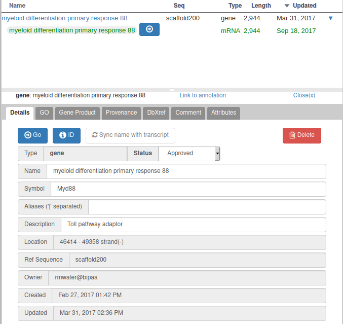
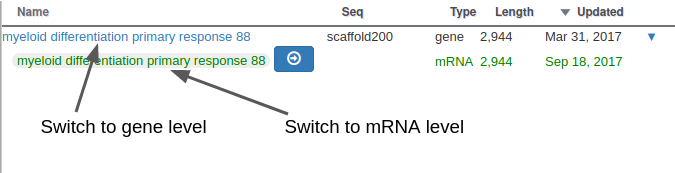
With Apollo, you can edit information at the gene level, or at the mRNA level. This is especially useful when you annotate a gene having multiple isoforms. When clicking on the “Open Annotation” menu, the panel above concerns the gene level information. You can switch to between the gene and mRNA level by clicking on the gene/mRNA names:

If the gene you are annotating does not have multiple isoforms , you should only care about the gene level information. The empty fields at the mRNA level will be automatically copied from the gene information when releasing subsequent OGS releases.

For each gene, we ask you to at least :

Give a name (human readable long name, e.g. : gluthatione s-transferase )
Give a symbol (must be unique, must not contain space, “ _” is allowed, e.g.: GST or GR154 )
Assign a status to the gene
Assign the gene to an annotation group (see below)

In the description field you can optionally add a longer description of the gene name if necessary (see example above).

Please pay a particular attention to the following points :

Follow the naming rules for your gene family (see “Gene nomenclature” below)
Name or symbol should not be ID (like DV0000000-RA ). BIPAA will manage the ID assigned to genes when releasing OGS.
Do not add any organism prefix such as “Dv-“
In most cases, when you have sufficient supporting evidences (RNASeq, Alignements, …) and/or the gene looks ok compared to orthologs, do not add “ putative ” to the gene name .
In borderline cases, when you are really not sure of the gene annotation (e.g. low sequence similarity) you can add “ putative ” to the gene name . Anyway, do not use “ similar to “, “ -like ” or any other synonym.
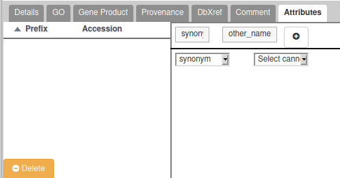
If the gene you are annotating have multiple possible names/symbols, use the preferred ones as the official name and symbol , and add the other ones in the “Attributes” section as synonyms: In the Tag column, select the “Synonym” which should appear in a drop-down list. In the “Value” column, write the alternate names or symbols. See the following screenshot for an example (click on the “+” to validate):

If the gene you are annotating have multiple isoforms , you should populate the mRNA form for each isoform, in particular :

Add a letter (A, B, C, …) at the end of the name to distinguish each isoform (e.g. : gluthatione s-transferase A )

Annotation status

There are 3 possible statuses for a gene:

Needs review : you have begun annotating this gene, but it’s not finished.
Approved : you consider the annotation finished for this gene (errors and warnings can still appear in the validation report, see below).
Deleted : if you want to permanently remove a gene in the next OGS. Typical usage is that an mRNA was predicted during the automatic annotation, but you are sure that there is no mRNA at this location. In this case, drag the problematic mRNA to the annotation track, copy the mRNA id in the name field (e.g. DV0000000-RA ) and set its status to Deleted . The mRNA will be removed in the next OGS. If the gene have multiple isoforms, other isoforms will be kept. Note that when you want to split a gene in multiple small genes, you don’t need to mark as deleted the original gene, it will be deleted automatically.

It is up to each group leader to decide who should approve each gene. In some groups the leader will choose to be the only one to approve a gene, in other groups the leader can decide to trust each annotator.

Annotation groups

Assigning genes to an annotation group is necessary to ease tracking of the progress of the annotation project. Groups are defined by the leader(s) of the project, and correspond to families of genes you have been assigned the annotation. Each group leader will be in charge of reporting/summarizing the scientific results of the annotation to the project leaders.

To assign a gene to a group, add a new Attribute in the “Attributes” section of the gene. In the first list, you must select “annotgroup” which should appear in a drop-down list. In the second list, select a value from the full list of annotation groups. Don’t forget to click on the “+” button to validate.

If you annotated a gene which belongs to no specific group, you have two solutions:

If you would like to annotate a new family of genes, get in touch with us and we will add a new group to the list after evaluating it with the project leaders.
A special “other” group is also available. It should only be used for a few genes you find interesting but are not specifically targeted by the annotation project.

You can also add more (optional) information for each gene:

Some external references (DBXrefs, e.g. UniProt ID) (DbXref tab)
Some publication using their PubMed ID (DbXref tab)
Gene Ontology terms: see below

These fields are not mandatory, but it’s always good to collect as much information as possible while annotating.

Gene Ontology terms

Gene Ontology terms allow to tag a gene with terms from a controlled vocabulary, corresponding to molecular functions, biological processes or cellular components.

Recently, Apollo introduced a new form to add GO terms to a gene. From the “GO” tab of a gene, click on the “New”, button. You will see a form looking like the following example screenshot:

Here’s the meaning of each field:

Aspect: select a Gene Ontology branch (MF for molecular functions, BP for biological processes or CC for cellular components)
Go Term: select the GO term to associate to the gene (write free text, a list of suggestions will appear)
Relationship between Gene Product and GO Term: select the kind of relation between the gene and the select GO Term
Not: check to reverse the selected relationship (e.g. not involved in)
Evidence: ECO ontology term describing why you want to associated a gene and a GO-Term (write free text, a list of suggestions will appear)
With: optional id of an element used as an evidence (in this example, the evidence is a similarity with the Q99836 UniProt record)
Reference: optional pubmed id of an article supporting your annotation
Note: free text comments

Don’t forget to hit the “Add” button when adding a “With” of “Note” element. The form should look like this before hitting the “Save” button:

Particular cases

Gene x is truncated on one end.

In case the gene you are annotating is not complete because it is on the 5′ or 3′ end of a scaffold, and you couldn’t find the other part of the gene on another scaffold, add the word “ Partial ” in the comment tab of the annotation editor.

Gene X is incomplete/missing an exon

In rare cases you may find that a gene is incomplete because some internal exon is missing, e.g. a 4 exons gene found on a single scaffold, but exon 3 is not present in the scaffold sequence.

In this case, you should create one gene model for each part of the gene, each one having a “ Part “ attribute (the value must be the number of the fragment, starting with 1 at the 5′ end of your gene) and the word “ Partial ” in the comment tab of the annotation editor.

Gene X is spread over 2 scaffolds

Because genomes can be very fragmented, it is often the case that your gene is not completely included in one unique scaffold. For these cases, you have to annotate separately the two fragments, but use the same name and symbol. For each part of the gene, you have to add an attribute in the “Annotation editor”. Select “ Part ” in the first column, and the value must be the number of the fragment, starting with 1 at the 5′ end of your gene.

Be careful if the end of the exon in the previous part does not stop at the end of a codon. You have to change consequently the translation start of the first exon int the next part.

If a part is missing between the 2 fragments, you should had the word “ Partial ” in the comment tab of the annotation editor for both fragments.

Gene Y is present in multi copy, caused by unassembled alleles

In some cases you can find 2 complete versions of the same gene of interest in the assembly. If you think that these 2 versions are not real duplications but the results of 2 unassembled alleles, annotate the 2 alleles, give them the same name and symbol but add the attribute “ Allele ” (tag column) with the value A or B.

Gene Z is spread over 2 scaffolds AND have multiple copies

Just add the 2 “Part” and “Allele” attributes for each fragment/copy.

How automatic and manual annotation will be merged?

The merging is done by looking at overlaps on CDS of automatic and manually annotated genes. In most cases this proved to work well on other genome projects. If you encounter more exotic situations (e.g. you want to replace a specific gene from the automatic annotation, or you want to keep both automatic and manually annotated gene), please contact us and we will guide you on how to properly annotate it.

Correcting the genome sequence

While annotating a gene, if you think the genome sequence is wrong and that the gene you’re annotating is impacted (e.g. wrong ORF), you have the possibility to add alterations to the sequence (insertions, deletions, mutations). Please make these corrections only if the sequence modification is well supported (by RNASeq for example). Also keep in mind that, while at some point in the future we could use this information to generate new versions of the genome assembly at the same time as new OGS release, this is not currently the case. It will only allow you to export correct transcript and protein sequences for the affected genes.

Gene nomenclature

Giving correct names and symbols is important, but not always easy.

Some gene families have very well established rules to assign gene names (e.g. based on orthology with model species). In this case, annotators should follow these rules.

In other gene families where no consensus has been made in the scientific community, annotation group leaders should define rules to name the annotated genes. These rules should be clearly defined, and documented on this page . Please contact us if you want to add rules for a new gene family.

Validation of the annotation

To check that your favorite genes were correctly annotated, a report is available following the “Annoration report” link in the top menu.

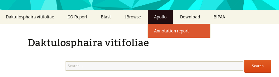
It is updated every night, and it contains the list of genes that you created. Each gene can be associated with some warnings and/or errors .

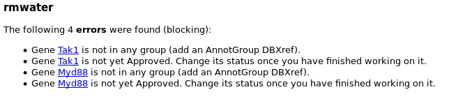
Errors are things you must correct to make your gene correctly annotated. Genes with errors will not be included in the next OGS release.

Warnings are minors hints we give you because we found something potentially wrong in the annotated gene. You should double check that everything is ok with this gene. Genes with warnings are included in the next OGS release.

Finally, hopefully, most of your genes will be ok . In this case, we will be able to include them in the next OGS release.

Please not that only Approved genes will be included in the next OGS release.

Our Culture
Open and FAIR Data
Research projects
Publications
Cellular Genomics
Decoding Biodiversity
Delivering Sustainable Wheat
Earlham Biofoundry
Transformative Genomics
Scientific Groups Our groups work at the forefront of life science, technology development, and innovation.
High-Performance Sequencing Dedicated and efficient high-throughput genomics led by experts in sequencing and bioinformatics.
Single-cell and Spatial Analysis Platforms to support single- or multi-cell analysis, from cell isolation, to library preparation, sequencing and analysis.
Earlham Biofoundry Providing expertise in synthetic biology approaches and access to laboratory automation
Tools and resources Explore our software and datasets which enable the bioscience community to do better science.
Cloud Computing Infrastructure for Data-intensive Bioscience
Web Hosting for Sites, Tools and Web Services
Earlham Enterprises Ltd
Events Calendar Browse through our upcoming and past events.
About our training High-quality, specialist training and development for the research community.
Year in industry Supporting undergraduate students to develop skills and experience for future career development.
Internships and opportunities Opportunities for the next generation of scientists to develop their skills and knowledge in the life sciences.
Immersive visitors A bespoke, structured training programme, engaging with the faculty, expertise and facilities at the Earlham Institute.
News Catch up on our latest news and browse the press archive.
Articles Explore our science and impact around the world through engaging stories.
Impact Stories Find out how we are contributing to the major challenges of our time.
Impact Through Policy Advocacy Engaging across the political spectrum to exchange knowledge and inform public policy.
Public engagement and outreach Communicating our research to inspire and engage learning.
Communications at EI We work across digital, multimedia, creative design and public relations to communicate our research.
Our Vision and Mission
Inclusivity, diversity, equality and accessibility
Scientific Advisory Board
Our Management Team
Operations Division
Careers overview
Postgraduate Studies
Group leaders
Fellowships
Life at Earlham Institute
Living in Norfolk

Why is genome annotation important?

Genome annotation is no simple feat, but it’s incredibly important in identifying the functional elements of DNA. Building the appropriate tools and pipelines is key.

With expertise gleaned from working with a diverse range of genomes - from aphids to wheat, and protists to fish - Earlham Institute scientists explain how genome annotation has advanced over the years, and why it is so important.

Gemy Kaithakottil is celebrating his tenth anniversary at the Earlham Institute this February, having helped to oversee a decade of dramatic transformation in how we annotate genomes.

“We’ve come a long way in the last ten years. Back then, before we began, the process was more like running software and scripts one by one. Now, we’ve merged everything into a streamlined pipeline and shaved a lot of time off the process.”

Throughout that time, Kaithakottil has worked as a Senior Bioinformatician and Software Developer in the Swarbreck Group , developing a suite of tools and pipelines that help us to more accurately map where genes lie along a genome.

We’ve come a long way in the last ten years. Back then, before we began, the process was more like running software and scripts one by one. Now, we’ve merged everything into a streamlined pipeline and shaved a lot of time off the process.

What is a genome annotation?

Simply put, genome annotation involves taking genomic data - DNA or RNA sequences - and mapping the correct genes (or more accurately, functional elements) to the correct locations. It gives the genome meaning.

According to Kaithakottil, this is an essential step that is frustratingly undervalued.

“People often spend a lot of effort on genome assembly, but eventually the research is going to work with the protein or the functional parts of it. If you're not going to give any effort to that part, then what's the point?

“You have to put equal - or even more effort - into the annotation.”

This can be done manually, by looking directly at the data and identifying the precise starting points of genes, but that takes a lot of time.

“When I was working at the Sanger Institute on the Human Genome Project, we annotated the human genome by going gene by gene across every chromosome,” says Dr David Swarbreck, Core Bioinformatics Group Leader at the Earlham Institute.

“We used manual annotation tools to visually examine alignments of cDNAs and proteins and, based on these, we could construct gene-models to define a gene's structure. This was a huge team effort and manual curation to this extent is not possible for most newly-sequenced and assembled genomes.

“I wanted something compatational that would work in a similar way to a manual annotator, enable us to assess alternative gene models, generate metrics to aid that comparison and make choices over the models we include or exclude: allowing us to shape the annotation for specific projects but without us having to do it manually.”

Genome Annotation Workshop 2022

You can learn from the experts how to annotate a genome at this year’s training workshop, delivered by the Core Bioinformatics Group here at the Earlham Institute.

Date: 17 - 19 May 2022

Moving towards genome annotation pipelines

One of the first genomes annotated by Swarbreck and his group was that of the green peach aphid , Myzus persicae , in a collaboration with the Hogenhout Group at the John Innes Centre that continues to this day.

“We played around with all the available tools at the time, to see what was available,” says Swarbreck. “The problem was, many of the more comprehensive pipelines weren’t easy to translate to running in your own environment.”

Kaithakottil adds that, “with any new pipeline, you need to understand the software, then work out what parameters you need to use, or tweak, for a particular species. It's not one size fits all. You need to understand the species that you're working with.”

As those early, non-human genomes were being assembled and annotated, RNA-seq data from transcriptome sequencing - the potentially expressed functional elements - was becoming more prevalent. So, too, were longer reads from the sequencers.

“We found that there was quite a bit of variation between different methods and different ways of dealing with that data,” says Swarbreck. “We concluded that there was no single tool out there that we found worked for all situations.

“We were looking for something that would allow us to try to integrate results of all these different transcriptome assemblers.”

With any new pipeline, you need to understand the software, then work out what parameters you need to use, or tweak, for a particular species. It's not one size fits all. You need to understand the species that you're working with.

Genome annotation pipelines at the Earlham Institute

That led to the development of Mikado and Portcullis , which were essential tools in the huge global effort to sequence, assemble and annotate the genome of bread wheat - a major milestone for such a crucial source of food.

Mikado is a tool, according to a former developer Dr Luca Venturini, based on the traditional stick game that is its namesake, aiming to “imagine genes as sticks and to capture the ones with the highest value without getting the others.”

What Mikado does, essentially, is find more real genes - filtering out false positives and identifying where there might have been false negatives. An example would come from gene duplications, whereby some software may have accidentally identified two very similar genes as only one.

“At the time we were working as part of the International Wheat Genome Sequencing Consortium and wanted a transparent approach that would enable us to integrate two alternative gene sets created by our collaborators,” says Swarbreck. “We made some tweaks to Mikado, and used it as a method to bring these two gene sets together, essentially cherry picking the ‘better’ models from the two annotations.”

Since then, the group has been integral to many genome sequencing projects, from various plant and tree species through to insects, fish, rodents, fungi and numerous others.

Now, the aim is to integrate these tools to tackle the biggest prize of all - the Darwin Tree of Life Project that aims to sequence the DNA of all eukaryotic life in the UK.

People often spend a lot of effort on genome assembly, but eventually the research is going to work with the protein or the functional parts of it. If you're not going to give any effort to that part, then what's the point? You have to put equal - or even more effort - into the annotation.

Reat: an all-encompassing, easy-to-use genome annotation pipeline

“We've got a growing number of projects and collaborations that use these tools, but what we have aimed for all along is an easy to run, all-encompassing annotation pipeline,” says Swarbreck. “The solution to that was to develop what we’ve called the reat toolkit.”

That toolkit was most recently used in an effort to produce the best ever reference genome for tilapia - a fish of exceptional importance in global aquaculture. It helped bioinformatician Dr Will Nash produce a comprehensive genome annotation.

Reat contains a module for dealing with a whole variety of transcriptome data, including cDNA, PacBio, nanopore, and short reads, and there are different workflows for those different types of data as well.

There's also a module for dealing with homology data from protein alignments, together with a gene prediction module - and at the end of that a consolidated gene annotation across all these different methods.

“Rather than try to generate a single set of models for each project, we generate lots of different gene models through different routes,” explains Swarbreck. “We then use our Minos pipeline to bring these all together and select the final ‘best’ models.

“Rather than putting all our eggs in one basket, we accept that it’s best to vary parameters, the choice of tools, and the inputs into these tools. We can achieve a higher quality final annotation and have an approach that is more robust across projects by generating alternative gene models.

“Ultimately, you need to have some way of making a final selection. Minos provides us with a means of making that selection that we can control, allowing us to review and tweak as required.”

How can I access genome annotation tools and expertise at the Earlham Institute?

The reat pipeline is available to anyone who would like to use it, open-source, on GitHub. The same is true of mikado, portcullis, minos and a range of other tools and pipelines for genome annotation.

“We are more than happy to keep in touch with anyone interested in using these pipelines,” says Kaithakottil. “People tend to ask questions in the issues section of GitHub, and we gladly help them there. We’ll reply to emails, too, of course!”

There’s also a training course on Genome Annotation , which Kaithakottil would encourage those looking to make use of these pipelines to sign up for.

“The workshop starts from the very basics,” he explains. “We introduce participants to genome annotation and then go through a number of pipelines, including our own, such as Mikado and Minos, as well as some external pipelines.

“We go through using metrics, best practice, explore the parameters you should be using - and then how to run and install these tools, and how to use them most effectively. Thanks to CyVerse UK , trainees can also access the resources via virtual machines to see their outputs, tweak parameters, and modify them to improve their results.”

If you’d like to sign up for the workshop in 2022, registrations end on April 17. Keep your eyes on the events calendar, which is regularly updated, for future events, or sign up to the Earlham Institute monthly newsletter.

This 3-day course will help to provide scientists with an overview of eukaryotic genome annotation approaches, covering advances in Next Generation Sequencing (NGS) technologies, transcriptome assembly, best practice guidance for building gene models utilising short and long read sequencing data or cross species proteins, how to integrate and assess different gene models and create a publication/release ready gene set.

Course Dates: 17 - 19 May 2022
Time : 09.30 - 15.00
Venue : Online (via Zoom)
Registration Deadline: 17 April 2022
Registration Cost : £150.00

Precision genome annotation: Portcullis and Mikado

Generating a high-quality tilapia genome assembly: from sample to sequence

How our tools can help you: Mikado

Scientific Groups
High-Performance Sequencing
Single-cell and Spatial Analysis
Tools and resources
Events Calendar
About our training
Year in industry
Internships and opportunities
Immersive visitors
Impact Stories
Impact Through Policy Advocacy
Public engagement and outreach
Communications at EI

Warning: The NCBI web site requires JavaScript to function. more...

An official website of the United States government

The .gov means it's official. Federal government websites often end in .gov or .mil. Before sharing sensitive information, make sure you're on a federal government site.

The site is secure. The https:// ensures that you are connecting to the official website and that any information you provide is encrypted and transmitted securely.

Publications
Account settings

Integrated reference sequences

Eukaryotic Annotation Home
Annotation Process
NCBI Handbook Chapter
Software Release Notes
All Annotated Genomes
Recently Annotated Genomes
Annotation Runs In Progress
Annotations Per Year Graphs
Annotation Policy
Request Annotation

The NCBI Eukaryotic Genome Annotation Pipeline

The NCBI Eukaryotic Genome Annotation Pipeline provides content for various NCBI resources including Nucleotide , Protein , BLAST , Gene and the Genome Data Viewer genome browser.

This page provides an overview of the annotation process. Please refer to the Eukaryotic Genome Annotation chapter of the NCBI Handbook for algorithmic details.

The pipeline uses a modular framework for the execution of all annotation tasks from the fetching of raw and curated data from public repositories (sequence and Assembly databases) to the alignment of sequences and the prediction of genes, to the submission of the accessioned annotation products to public databases. Core components of the pipeline are alignment programs ( Splign and ProSplign ) and an HMM-based gene prediction program ( Gnomon ) developed at NCBI.

Important features of the pipeline include:

flexibility and speed
higher weight given to curated evidence than non-curated evidence
utilization of RNA-Seq for gene prediction
production of models that compensate for assembly issues
tracking of gene loci from one annotation to the next
ability to co-annotate multiple assemblies for the same organism

The products of an annotation run (chromosome, scaffolds and model transcripts and proteins) are labeled with an Annotation Name. There are two formats for the Annotation Name, which is used throughout NCBI as a way to uniquely identify annotation products originating from the same annotation run.

the combination of the organism name and Annotation Release number (e.g. NCBI Pongo abelii Annotation Release 103)
the combination of the RefSeq assembly accession and the year and month in which the annotation was started (e.g. NCBI GCF_016801865.2-RS_2022_12)

Source of genome assemblies

Transcript alignments, transcriptomics long read alignments, rna-seq read alignments, protein alignments, model prediction, curated refseq genomic sequence alignments, choosing the best models for a gene, protein naming and determination of locus type, gene ontology, assignment of geneids, annotation of small rnas, annotation of transcription start sites (tss), special considerations, annotation of multiple assemblies, re-annotation, annotation quality, annotation products, data availability.

Please see The Eukaryotic Genome Annotation chapter in the NCBI Handbook for more details about the algorithms.

The figure below provides an overview of the annotation process. The genomic sequences are masked (grey) and transcripts (blue), proteins (green) and RNA-Seq reads and, if available in SRA, long reads transcriptomes and Cap Analysis Gene Expression (CAGE) data (orange) are aligned to the genome. If available for the organism being annotated, curated RefSeq genomic sequences are also aligned (pink). Gene model prediction based on transcript and protein alignments is then performed (brown). The best models are selected among the RefSeq and the predicted models, named and accessioned (purple). Finally, the annotation products are formatted and deployed to public resources (yellow).

The RefSeq assemblies that are annotated by NCBI are copies of the genome assemblies that are public in INSDC ( DDBJ , ENA and GenBank ). Unplaced scaffolds with length below 1000 bases may not be included in the RefSeq copy of the assembly if the INSDC assembly contains more than 300,000 unplaced scaffolds and more than 25,000 of them are below 1000 bases. Both RefSeq and GenBank assemblies are further described in the Assembly resource.

Masking is done using RepeatMasker or WindowMasker . Human and mouse are masked with RepeatMasker using their respective Dfam libraries, while genomes from other species are masked with WindowMasker .

The set of transcripts selected for alignment to the genome varies by species, and may include transcripts from other organisms. This set generally includes:

Known RefSeq transcripts: Coding and non-coding RefSeq transcripts with NM_ or NR_ prefixes, respectively, are generated by NCBI staff based on automatic processes, manual curation, or data from collaborating groups (see more details here )
GenBank transcripts from the taxonomically relevant GenBank divisions, and the Third-Party Annotation ( TPA ), High-throughput cDNA (HTC) and Transcriptome Shotgun Assembly ( TSA ) divisions
ESTs from dbEST

Sequences highly likely to be mitochondrial or to have cloning vector or IS element contamination, and sequences identified as low quality by RefSeq curation staff are screened out.

RefSeq transcripts and non-RefSeq transcripts that pass the contamination screen are aligned locally to the genome using BLAST to identify the location(s) at which transcripts align. Global re-alignment at these locations is performed with Splign to refine the identification of splice sites. Alignments are then ranked and filtered based on customizable criteria (such as coverage, identity, rank). Typically, only the best-placed (rank 1) alignment for a given query is selected for use in the downstream steps.

Transcriptomics reads from SRA generated using long read sequencing technologies such as PacBio or Oxford Nanopore are aligned to the genome using Minimap2 . Each transcript's best-placed (rank 1) alignment is selected for use in the downstream steps, if above 85% identity.

RNA-Seq reads for the species or closely related species are aligned to the genome. When a very large number of samples and reads (multiple billions) are available in SRA , projects with samples spanning the widest range of tissues and developmental stages are chosen over others, with a preference for untreated or non-diseased samples. RNA-Seq reads are aligned to the genome with STAR . To address the short length, redundancy and abundance of the reads, alignments with the same splice structure and the same or similar start and end points are collapsed into a single representative alignment. Information is recorded about the samples and number of reads represented by each alignment, so the level of support can be used to filter alignments and evaluate gene predictions. Alignments representing very rare introns likely to be background noise are filtered out.

For each SRA run aligned to the genome, RNA-seq read coverage graphs in UCSC BigWig format are generated and made available for download on the FTP site (see link below). The number of reads mapped to annotated genes is also counted using Subread featureCounts software, and the gene expression counts files are made available for download on the FTP site. Additionally, a file containing information about all of the SRA runs used is provided.

The set of proteins selected for alignment to the genome varies by species, and may include proteins from other organisms. This set generally includes:

Known RefSeq proteins
GenBank proteins derived from cDNAs from the taxonomically relevant GenBank divisions

Highly repetitive sequences are removed from the set. Proteins are aligned locally to the genome with BLAST and re-aligned globally using ProSplign . Alignments are then ranked and filtered based on customizable criteria.

Protein, transcript, transcriptomics and RNA-Seq read alignments are passed to Gnomon for gene prediction. Gnomon first chains together non-conflicting alignments into putative models. In a second step, Gnomon extends predictions missing a start or a stop codon or internal exon(s) using an HMM-based algorithm. Gnomon additionally creates pure ab initio predictions where open reading frames of sufficient length but with no supporting alignment are detected.

This first set of predictions is further refined by alignment against a subset of the nr (non-redundant) database of protein sequences. The additional alignments are added to the initial alignments, and the chaining and ab initio extension steps are repeated. The results constitute the set of Gnomon predictions.

Gnomon predictions may include deletions or insertions of Ns with respect to the genomic sequence. These differentes are introduced to compensate for frameshifts or stop codons in the literal translation of the genome, when the aligning proteins provides evidence of an intact ORF.

For some organisms, a set of genomic sequences is curated ( RefSeq accessions with NG_ prefixes). These sequences represent either non-transcribed pseudogenes, a manually annotated gene cluster that is difficult to annotate via automated methods, and human RefSeqGene records. They are aligned to the genome, and their best placement is identified.

The final set of annotated features comprises, in order of preference, pre-existing RefSeq sequences and a subset of well-supported Gnomon -predicted models. It is built by evaluating together at each locus the known RefSeq transcripts, the features projected from curated RefSeq genomic alignments and the models predicted by Gnomon .

1. Models based on known and curated RefSeq

RefSeq transcripts are given precedence over overlapping Gnomon models with the same splice pattern. Alignments of known same-species RefSeq transcripts or curated genomic sequences are used directly to annotate the gene, RNA and CDS features on the genome. Since the RefSeq sequence may not align perfectly or completely to the genomic sequence, a consequence of this rule is that the annotated product may differ from the conceptual translation of the genome. Differences between the RefSeq transcripts and the genome are provided in a note on the RefSeq genomic record (scaffold or chromosome).

2. Models based on Gnomon predictions

Gnomon predictions are included in the final set of annotations if they do not share all splice sites with a RefSeq transcript and if they meet certain quality thresholds including:

Only fully- or partially-supported Gnomon predictions, or pure ab initio Gnomon predictions with high coverage hits to UniProtKB/SwissProt proteins are selected
When multiple fully-supported transcript variants are predicted for a gene, only the Gnomon predictions supported in their entirety by a single long alignment (e.g. a full-length mRNA) or by RNA-Seq reads from a single BioSample are selected
Poorly-supported Gnomon predictions conflicting with better-supported models annotated on the opposite strand are excluded from the final set of models
Gnomon predictions with high homology to transposable or retro-transposable elements are excluded from the final set of models

3. Integrating RefSeq and Gnomon annotations

As a result of the model selection process, a gene may be represented by multiple splice variants, with some of them known RefSeq and others model RefSeq (originating from Gnomon predictions).

Gnomon predictions selected for the final annotation set are assigned model RefSeq accessions with XM_ or XR_ prefixes for transcripts and XP_ prefixes for proteins to distinguish them from known RefSeq with NM_/NR_ and NP_ prefixes. Model RefSeq can be searched in Entrez with the query “srcdb_refseq_model[properties]” while known RefSeq sequences can be obtained with the query “srcdb_refseq_known[properties]”.

Genes represented by known or curated RefSeq sequences inherit the Gene symbol, name and locus type (e.g. coding, pseudogene...) of the RefSeq sequence.
Genes represented by predicted models are named based on homology to SwissProt proteins.
Most Gnomon models with insertions, deletions or frameshifts are labeled pseudogenes.
Gnomon models with insertions or deletions relative to the genome may be considered coding if they have a strong unique hit to the SwissProt database or appear to be orthologs of known protein-coding genes. Titles for these models are prefixed with “PREDICTED: LOW QUALITY PROTEIN” to indicate that these models and the underlying assembly sequences may content defects.
Gnomon models that appear to be single-exon retrocopies of protein-coding genes may be annotated as pseudogenes.
When multiple assemblies are annotated , a partial or imperfect model may be called coding because a complete model exists at the corresponding locus on one of the other annotated assemblies.

Gene Ontology (GO) terms for all annotated proteins were computed using InterProScan , a tool that identifies protein domains and families. The GO terms were then collated by gene, and the resulting GO annotations are made available for download from the FTP site (see link below) in the GAF (GO Annotation File) format .

Genes in the final set of models are assigned GeneIDs in NCBI's Gene database.

A gene represented by a known RefSeq transcript will receive the GeneID of the RefSeq transcript.
All alternative splice forms of a gene get the same GeneID.
As much as possible, GeneIDs are carried forward from one annotation run to the next, using the mapping of the new assembly to the previous one if the assembly was updated.
Gene features mapped to equivalent locations of co-annotated assemblies are assigned the same GeneIDs.
miRNAs are imported from miRBase , accessioned with NR_ prefixes and placed using Splign .
tRNAs are predicted with tRNAscan-SE .
Starting with software version 8.0, rRNAs, snoRNAs and snRNAs are annotated by searching eukaryotic RFAM HMMs against the genome with Infernal's cmsearch .

Starting with software release 9.0, Cap Analysis Gene Expression (CAGE) data that is available in SRA for the species are aligned to the genome with Splign and used for annotating transcription start sites.

When multiple assemblies of good quality are available for a given organism, annotation of all is done in coordination. To ensure that matching regions across assemblies are annotated the same way, assemblies are aligned to each other before the annotation.

Assembly-assembly alignment results are used to rank the transcript and the curated genomic alignments: for a given query sequence, alignments to corresponding regions of two assemblies receive the same rank.
Corresponding loci of multiple assemblies are assigned the same GeneID and locus type.

Organisms are periodically re-annotated when new evidence is available (e.g. RNA-Seq) or when a new assembly is released. Special attention is given to tracking of models and genes from one release of the annotation to the next. Previous and current models annotated at overlapping genomic locations are identified and the locus type and GeneID of the previous models are taken into consideration when assigning GeneIDs to the new models. If the assembly was updated between the two rounds of annotation, the assemblies are aligned to each other and the alignments used to match previous and current models in mapped regions.

The quality of the annotation is assessed prior to publishing, based on the intrinsic characteristics of the annotated models and on the expectations for the species. Indicators of a low quality annotation may disqualify a genome from being included in RefSeq. These indicators are: high count of coding genes that lack near-full coverage by alignments of experimental evidence, high count of partial coding genes (lacking a start or stop codon, or internal exons), high count of low-quality genes with suspected frameshifts or premature stop codons, low BUSCO completeness score (see below), and, for vertebrates, low count of genes with orthologs to a reference species.

BUSCO run in "protein" mode provides an estimate of the completeness of the gene set. The BUSCO models (single-copy marker genes) for the most fitting lineage based on NCBI Taxonomy are searched against the longest protein for each annotated coding gene. Results are reported in BUSCO notation (C:complete [S:single-copy, D:duplicated], F:fragmented, M:missing, n:number of genes used).

The scaffolds and chromosomes of the assembled genomes, with the annotation products as features.
The individual products (transcripts and proteins)

Product	Origin of the product	Note for the features on the scaffolds and chromosomes*
Known transcripts/proteins (NM_, NR_, NP_)	curated RefSeq genomic	"Derived by automated computational analysis using gene prediction method: Curated Genomic"
Known transcripts/proteins (NM_, NR_, NP_)	known RefSeq transcript	"Derived by automated computational analysis using gene prediction method: BestRefseq"
Model transcripts/proteins (fully or partially supported) (XM_, XR_, XP_)	Gnomon	"Derived by automated computational analysis using gene prediction method: Gnomon"
Model short non-coding transcripts (XR_)	Rfam + cmsearch	"Derived by automated computational analysis using gene prediction method: cmsearch"
tRNAs (no accession)	tRNAscan-SE	"tRNA features were annotated by tRNAscan-SE"
Non-transcribed pseudogenes (no accession)	curated RefSeq genomic	"Derived by automated computational analysis using gene prediction method: Curated Genomic"
Non-transcribed pseudogenes (no accession)	Gnomon	"Derived by automated computational analysis using gene prediction method: Gnomon"
Full set of Gnomon predictions (no accession)	Gnomon	NA. Not in the sequence database. Available on the and as databases

Sequence records for predicted models, scaffolds and chromosomes contain the Annotation Name, which uniquely identifies the annotation. Examples:

The sequence records for scaffolds, chromosomes and predicted transcripts and proteins for NCBI Pongo abelii Annotation Release 103 contain the following comment:

##Genome-Annotation-Data-START## Annotation Provider :: NCBI Annotation Status :: Full annotation Annotation Name :: Pongo abelii Annotation Release 103 Annotation Version :: 103 Annotation Pipeline :: NCBI eukaryotic genome annotation pipeline Annotation Software Version :: 8.0 Annotation Method :: Best-placed RefSeq; Gnomon Features Annotated :: Gene; mRNA; CDS; ncRNA ##Genome-Annotation-Data-END##

The sequence records for scaffolds, chromosomes and predicted transcripts and proteins for NCBI GCF_016801865.2-RS_2022_12 contain the following comment:

##Genome-Annotation-Data-START## Annotation Provider :: NCBI RefSeq Annotation Status :: Full annotation Annotation Name :: GCF_016801865.2-RS_2022_12 Annotation Pipeline :: NCBI eukaryotic genome annotation pipeline Annotation Software Version :: 10.1 Annotation Method :: Gnomon; cmsearch; tRNAscan-SE Features Annotated :: Gene; mRNA; CDS; ncRNA ##Genome-Annotation-Data-END##

The data produced by the annotation pipeline is available in various resources:

Genome Data Viewer
BUSCO : Manni M et al. Molecular biology and evolution 2021, 38 (10):4647-4654
InterProScan : Jones P et al. Bioinformatics 2014. 30 (9):1236-1240
Minimap2 : Li H. Bioinformatics 2018 34 (18):3094-3100
miRBase : Griffiths-Jones S. Nucleic Acids Research 2004, 32 (Database Issue):D109-11
RefSeq : Pruitt KD et al. Nucleic Acids Research 2014, 42 (Database issue):D756-63
RepeatMasker : Smit AFA, Hubley R, Green P. RepeatMasker Open-3.0. 1996–2004. http://www.repeatmasker.org
Rfam : Nawrocki, EP et al. Nucleic Acids Research 2015, 43 (Database issue):D130-7
Splign : Kapustin Y, Souvorov A, Tatusova T, Lipman D. Biology Direct 2008, 3 :20
STAR : Dobin A, Davis CA, Schlesinger F, Drenkow J, Zaleski C, Jha S, Batut P, Chaisson M, Gingeras TR. Bioinformatics 2013, 29 (1): 15–21
Subread featureCounts : Liao, Y, Smyth GK, Shi, W. Bioinformatics 2014, 30 (7):923-930
tRNAscan-SE : Lowe, TM and Eddy, SR. Nucleic Acids Research 1997, 25 : 955-964
WindowMasker : Morgulis A, Gertz EM, Schäffer AA, Agarwala R. Bioinformatics 2006 2 :134-41

Connect with NLM

National Library of Medicine 8600 Rockville Pike Bethesda, MD 20894

Web Policies FOIA HHS Vulnerability Disclosure

Help Accessibility Careers

Last updated: 2024-04-04T20:39:01Z

Bioinformatics
Agriculture
Gene Therapy
Medical Devices

Select Page

What is Gene Annotation in Bioinformatics?

Posted by Biolyse | Nov 3, 2018 | Bioinformatics | 0 |

Over the years scientist and researchers have made tremendous efforts through various inventions and innovation to make life better. Bioinformatics as an interdisciplinary approach has created numerous opportunities in scientific advancements and promoted efforts towards the realization of better living. A considerable milestone development in bioinformatics goes down to the necessary level of life: genes. Previously identification and ability to distinguishing genes were limited hindering scientific manipulations and diagnostic procedures. With a clear understanding of the gene sequencing process, we can surely achieve massive success in the management of various conditions and generally maintaining a healthy generation. Gene annotation has made this to be in reach.

What is gene annotation?

In molecular biology, genomes make the basic genetic material and typically consist of DNA. Whereby, genome include the genes (coding) and the non-coding regions, of interest to us, are the coding regions as they actively influence basic life processes. The genes contain useful biological information that is required in building up and maintaining an organism. Gene annotation can be defined merely as the process of making nucleotide sequence meaningful. However, it’s a much complex process encompassing several procedures and a broad range of activities.

Gene annotation involves the process of taking the raw DNA sequence produced by the genome-sequencing projects and adding layers of analysis and interpretation necessary to extracting biologically significant information and placing such derived details into context. Through the aid of bioinformatics, there exists software to perform such complex procedures. The first gene annotation software system was developed in1995 at The Institute for Genomic Research, and this was used to sequence and analyze the genes of the bacterium Haemophilus influenza.

As a process of identification of gene location and coding regions, gene annotation helps us have an insight of what these genes do in the body by establishing structural aspects and relating them to functions of different proteins. Currently, the process is automated, and the National Center for Biomedical Ontology have a database for records and to enable comparison.

Learn More: How to Learn Bioinformatics Why is Bioinformatics important in Genetic Research? How to Get Into Bioinformatics

How is gene annotation performed?

Gene annotation can either be manual or electronic with the aid of tools developed by an amalgamation of organizations. The downsides of the manual technique are that it is time-consuming and the turn-over rate is much low. However, it remains useful for predictive purposes thus serves a complementary function. There exist three main steps in the process of gene annotation:

Identification of the non-coding regions of the genome (exons). This is vital to limit the range of analysis and only focus on the essential components as it is needless doing the tedious work on portions that give no or little biological information.

Gene prediction; these give an overview of the amino acid components of the genes and the role of such elements. Also referred to as gene finding, this process identifies regions of genomic DNA that encode genes. Empirical methods or Ab Initio methods can do it.

Establishing a connection and a correlation between the identified elements and the biological information at hand. Linking of biological functions and data is possible this way.

Homology-based tools for example Blast has hugely simplified the process of gene annotation, and this can now be done without much hassle as witnessed in manual methods that require human expertise.

Modalities of gene annotation

Genomics is a broad study and can be subdivided as structural genomics, functional genomics, and comparative genomics to leverage the understanding of this crucial topic. Similarly, gene annotation exists as a double-phased entity comprising of structural gene annotation and functional gene annotation.

Structural annotation

The initial process in gene annotation and involve identification by physical appearance, chemical composition, molecular weight variations, and general morphology. Such differences as coding regions, gene structures, ORFs and their locations , as well as regulatory motifs, are crucial information that is derived from this procedure and influence the process of gene identification as well as distinction. The accuracy of this process can be evaluated based on two parameters; specificity and accuracy. Where sensitivity is the percentage of right signals predicted among all possible correct strengths while specificity refers to the proportion of right signal among all that are forecasted.

Functional annotation

The process of relating crucial biological functions to the genetic elements as depicted in the structural annotation step. Biochemical functions, physiological functions, involved regulations and interactions atop expressions are some of the critical roles that are often considered in DNA annotation.

The above steps can involve biological experiments as well as in silico analysis mimicking the internal conditions. A new method seeking to improve genomics annotation- Proteogenomics is currently in use, and it utilizes information from expressed proteins, such information is obtained from mass spectrometry.

Essential components

Gene annotation is a purposeful process, and some of the vital information that we seek to extract from this process include; CDs, mRNA, Pseudogenes, promoter and poly-A signals, mcRNA among others. Such elements are minute and identification may be hectic. Scientists have developed software and tools to aid the process and notable tools frequently used are; ORF detectors, promoter detectors and start/stop codon identifiers. Automation of this process has created enhanced accuracy, and now there exist large discrepancies between with the manually conducted procedures as gene sequencing is a dynamic topic.

After a successful gene annotation process, it is expected that the obtained information should be published, stored in the database and shared for research purposes.

Gene annotation is a new and exceedingly promising idea, much remains unfolded, and there is a lot of potentially beneficial areas that remains to be explored. Fortunately, many groups have invested in gene annotation, and new developments arise daily. Some of the ongoing projects on gene annotation include; Ensembl, GENCODE and GeneRIF among others. It is important to appreciate that modern literature gets published daily concerning this topic and it is prudent to keep updated.

DNA annotation reveals much of the information contained in the genomes therefore complete gene annotation is descriptive of organisms being and thus remains a milestone invention.

About The Author

Why is bioinformatics important in genetic research.

November 3, 2018

How To Learn Bioinformatics

September 27, 2018

How to get into Bioinformatics

Bacterial Genome Annotation

Overview Questions: Which genes are on a draft bacterial genome? Which other genomic components can be found on a draft bacterial genome? Objectives: Run a series of tool to annotate a draft bacterial genome for different types of genomic components Evaluate the annotation Process the outputs to formate them for visualization needs Visualize a draft bacterial genome and its annotations Requirements: Introduction to Galaxy Analyses Time estimation: 3 hours Level: Introductory Introductory Supporting Materials: Datasets Workflows FAQs instances Available on these Galaxies Known Working UseGalaxy.eu ✅ ⭐️ Galaxy@AuBi ✅ UseGalaxy.cz ✅ UseGalaxy.fr ✅ Containers docker_image Docker image Published: Feb 1, 2024 Last modification: Mar 13, 2024 License: Tutorial Content is licensed under Creative Commons Attribution 4.0 International License . The GTN Framework is licensed under MIT purl PURL : https://gxy.io/GTN:T00403 rating Rating: 1.0 (0 recent ratings, 1 all time) version Revision: 8

After sequencing and assembly, a genome can be annotated. It is an essential step to describe the genome.

Genome annotation consists in describing the structure and function of the components of the genome, by predicting, analyzing, and interpreting them in order to extract their biological significance and understand the biological processes in which they participate. Among other things, it identifies the locations of genes and all the coding regions in a genome ( structural annotation ) and determines what those genes do ( functional annotation ).

To illustrate the process to annotate a bacterial genome, we take an assembly of a bacterial genome (KUN1163 sample) generated by following a bacterial genome assembly tutorial from data produced in “Complete Genome Sequences of Eight Methicillin-Resistant Staphylococcus aureus Strains Isolated from Patients in Japan” ( Hikichi et al. 2019 ).

Methicillin-resistant Staphylococcus aureus (MRSA) is a major pathogen causing nosocomial infections, and the clinical manifestations of MRSA range from asymptomatic colonization of the nasal mucosa to soft tissue infection to fulminant invasive disease. Here, we report the complete genome sequences of eight MRSA strains isolated from patients in Japan.

Agenda In this tutorial, we will cover: Galaxy and data preparation Contig annotation Further structural annotation Plasmids Integrons IS (Insertion Sequence) elements Visualisation of the annotation Conclusion

Galaxy and data preparation

Any analysis should get its own Galaxy history. So let’s start by creating a new one and get the data (contig file from the assembly) into it.

Hands-on: Prepare Galaxy and data Create a new history for this analysis Tip: Creating a new history To create a new history simply click the new-history icon at the top of the history panel:

Rename the history

Tip: Renaming a history Click on galaxy-pencil ( Edit ) next to the history name (which by default is “Unnamed history”) Type the new name Click on Save To cancel renaming, click the galaxy-undo “Cancel” button If you do not have the galaxy-pencil ( Edit ) next to the history name (which can be the case if you are using an older version of Galaxy) do the following: Click on Unnamed history (or the current name of the history) ( Click to rename history ) at the top of your history panel Type the new name Press Enter

Import the contig file from Zenodo or from Galaxy shared data libraries:

Tip: Importing via links Copy the link location Click galaxy-upload Upload Data at the top of the tool panel Select galaxy-wf-edit Paste/Fetch Data Paste the link(s) into the text field Press Start Close the window

Tip: Importing data from a data library As an alternative to uploading the data from a URL or your computer, the files may also have been made available from a shared data library : Go into Shared data (top panel) then Data libraries Navigate to the correct folder as indicated by your instructor. On most Galaxies tutorial data will be provided in a folder named GTN - Material –> Topic Name -> Tutorial Name . Select the desired files Click on Add to History galaxy-dropdown near the top and select as Datasets from the dropdown menu In the pop-up window, choose “Select history” : the history you want to import the data to (or create a new one) Click on Import

Contig annotation

Bakta is a tool for the rapid & standardized annotation of bacterial genomes and plasmids from both isolates and metagenome-assembled genomes (MAGs). It implements a comprehensive annotation workflow for coding and non-coding genes ( i.e. tRNA, rRNA).

Flow diagram of Bakta. It depicts the sequential steps and connections involved in its functioning.

It is also able to detect and annotate small proteins (sORF). Predicted CDS are annotated using an alignment-free protein sequence identification approach with cross-references to public databases via stable identifiers.

Hands-on: Contig annotation Bakta ( Galaxy version 1.8.2+galaxy0) with the following parameters: In “Input/Output options” : “The bakta database” : latest one “The amrfinderplus database” : latest one param-file “Select genome in fasta format” : Contig file In “Optional annotation” : “Keep original contig header (–keep-contig-headers)” : Yes In “Selection of the output files” : “Output files selection” : Annotation file in TSV Annotation and sequence in GFF3 Feature nucleotide sequences as FASTA Summary as TXT Plot of the annotation result as SVG

Bakta can generate many outputs. Here we selected:

Analysis_summary : a summary of the analysis as text file

Question How many contigs have been provided as input? How long is the draft genome? How many CDSs have been found? How many small proteins? Which other components have been found? How does it compare to results for KUN1163 in Table 1 in Hikichi et al. 2019 ? Solution 44 (the sequence count) 2,911,349 bp, with is a bit shorter than the expected 2,914,567 bp in Table 1 in Hikichi et al. 2019 2,717 CDSs, a bit more than the expected 2,704 CDSs in Table 1 in Hikichi et al. 2019 5 sORFs. There is no information about sORFs in Hikichi et al. 2019 Other components Components Bakta Hikichi et al. 2019 tRNAs 57 61 Transfer-messenger RNA (tmRNAs) 1 1 rRNAs 9 5 ncRNAs 95 No information

Nucleotide_sequences with feature nucleotide sequences as FASTA file

Question How many sequences are in this file? What are the sequences stored there? Solution 2,884 sequences Here are stored: tRNAs tmRNAs rRNAs ncRNAs CDSs sORFs

annotation_summary with annotations as simple human readble TSV

Question What is stored there? Solution This a table with 9 columns ( Sequence Id , Type , Start , Stop , Strand , Locus Tag , Gene , Product , DbXrefs ). It contains here 2,916 lines, so the information and location for: tRNAs tmRNAs rRNAs ncRNAs CDSs sORFs gaps oriCs oriVs oriTs

Annotation_and_sequences in GFF3

GFF is a file format used for describing genes and other features of DNA, RNA and protein sequences. It is a tab delimited file with 9 fields per line:

seqid : The name of the sequence where the feature is located.
source : The algorithm or procedure that generated the feature. This is typically the name of a software or database.
type : The feature type name, like “gene” or “exon”. In a well structured GFF file, all the children features always follow their parents in a single block (so all exons of a transcript are put after their parent “transcript” feature line and before any other parent transcript line). In GFF3, all features and their relationships should be compatible with the standards released by the Sequence Ontology Project.
start : Genomic start of the feature, with a 1-base offset. This is in contrast with other 0-offset half-open sequence formats, like BED.
end : Genomic end of the feature, with a 1-base offset. This is the same end coordinate as it is in 0-offset half-open sequence formats, like BED.
score : Numeric value that generally indicates the confidence of the source in the annotated feature. A value of “.” (a dot) is used to define a null value.
strand : Single character that indicates the strand of the feature. This can be “+” (positive, or 5’->3’), “-“, (negative, or 3’->5’), “.” (undetermined), or “?” for features with relevant but unknown strands.
phase : phase of CDS features; it can be either one of 0, 1, 2 (for CDS features) or “.” (for everything else). See the section below for a detailed explanation.
attributes : A list of tag-value pairs separated by a semicolon with additional information about the feature.

Question How many features are annotated? Solution 51k+ (number of lines in the GFF)

Plot of the annotation as circular genome annotation

A circular plot showcasing the draft genome, providing a visual representation of its genetic information.

Question What the 2 rings in the center? How are plotted the features? Solution The first ring represents the GC content per sliding window over the entire sequence(s) with in green representing GC above and red GC below average. The 2nd ring represents the GC skew in orange and blue. All features are plotted on two rings representing the forward and reverse strand from outer to inner with CDS in grey (the other colors are hard to distinguish)

Further structural annotation

Bakta gives a lot of information already, especially regarding CDSs or RNAs, but some structural annotation might be missing, e.g. plasmids, or interesting to identify independently.

To identify plasmids in our contigs, we use PlasmidFinder ( Carattoli and Hasman 2020 ), a tool for the identification and typing of plasmid sequences in Whole-Genome Sequencing. It uses the plasmidfinder database with hundreds of sequences to predict the plasmid in the data.

Hands-on: Plasmid identification PlasmidFinder ( Galaxy version 2.1.6+galaxy1) with the following parameters: In “Input parameters” : param-file “Choose a fasta or fastq file” : Contig file “PlasmidFinder database” : most recent one

PlasmidFinder generates several outputs:

raw_results.txt : A text file containing the result table and alignments

results.tsv : A tabular file with the following columns:

Plasmid : Plasmid against which the input genome has been aligned.
Identity : Percent identity in the alignment between the best matching plasmid in the database and the corresponding sequence in the inputgenome (also called the high-scoring segment pair (HSP)). A perfect alignment is 100%, but must also cover the entire length of the plasmid in the database (compare example 1 and 3).
Query/Template Length : Query length is the length of the best matching plasmid in the database, while HSP length is the length of the alignment between the best matching plasmid and the corresponding sequence in the genome (also called the high-scoring segment pair (HSP)).
Contig : Name of contig the plasmid is found in.
Position in contig : Starting position of the found gene in the contig.
Note : Notes about the plasmid
Accession number : Reference Genbank accession number accoding to NCBI for the plasmid in the database.

Question How many plasmid sequences have been found? Where are they located? Are these sequences all associated with Staphylococcus aureus ? What can we conclude about contig00019? Solution 5 plasmid sequences 3 are on the contig00019, 1 on contig00002, and 1 on contig00024 Looking at the accession number on the NCBI, we find that: CP000737, AP003139 (2 times) correspond to Staphylococcus aureus plasmids AF503772 corresponds to a Enterococcus faecalis plasmid CP003584 corresponds to a Enterococcus faecium plasmid All plasmid sequences corresponding to Staphylococcus aureus plasmids are all on contig00019, making this contig likely a plasmid. In addition, this contig has a length of 30,347 bp, which is similar to the expected length of the plasmid for KUN1163 in Table 1 in Hikichi et al. 2019

plasmid.fasta : A fasta file containing the best matching sequences from the query genome
hit_in_genome.fasta : A fasta file containing the best matching plasmid genes from the database

Integrons are genetic mechanisms that allow bacteria to adapt and evolve rapidly through the stockpiling and expression of new genes. An integron is minimally composed of:

a gene encoding for a site-specific recombinase (intI)
a proximal recombination site (attI), which is recognized by the integrase and at which gene cassettes may be inserted
a promoter (Pc) which directs transcription of cassette-encoded genes

To detect integrons, we will use IntegronFinder ( Néron et al. 2022 ). This tool:

Annotates the CDS with Prodigal

Detects independently:

integron integrase using the intersection of two HMM profiles: one specific of tyrosine-recombinase (PF00589) and one specific of the integron integrase, near the patch III domain of tyrosine recombinases
attC recombination sites with a covariance model (CM), which models the secondary structure in addition to the few conserved sequence positions.

Integrates the results to distinguish 3 types of elements

Complete integron: Integron with integron integrase nearby attC site(s)
In0 element: Integron integrase only, without any attC site nearby
CALIN element: Cluster of attC sites Lacking INtegrase nearby

Hands-on: Integron identification IntegronFinder ( Galaxy version 2.0.2+galaxy1) with the following parameters: param-file “Replicon file” : Contig file “Thorough local detection” : Yes “Search also for promoter and attI sites?” : Yes “Remove log file” : Yes

IntegronFinder generates 2 outputs:

A summary with for each sequence in the input the number of identified CALIN elements, In0 elements, and complete integrons.

Question How many integron elements have been found? Solution No integron elements have been found on any contig. It could be because the genome is too stable, or because the assembly quality is not good enough and some parts useful for the integron detection were removed.

An integron annotation file as a tabular

IS (Insertion Sequence) elements

Insertion sequence (IS) element is a short DNA sequence that acts as a simple transposable element. IS are the smallest but most abundant autonomous transposable elements in bacterial genomes. They only code for proteins implicated in the transposition activity. They play then a key role in bacterial genome organization and evolution.

To detect IS elements, we will use ISEScan ( Xie and Tang 2017 ). ISEScan is a highly sensitive software pipeline based on profile hidden Markov models constructed from manually curated IS elements

Hands-on: IS identification ISEScan ( Galaxy version 1.7.2.3+galaxy0) with the following parameters: param-file “Genome fasta input” : Contig file

ISEScan generates several files:

A summary as a table

The results as a table

Question How many IS elements have been detected? Where are they located? What the different IS families? Solution 20 Using Group data by a column to group and count on 1st column, we find: Contig IS element number contig00001 2 contig00002 1 contig00003 2 contig00004 1 contig00005 1 contig00006 1 contig00009 3 contig00010 1 contig00011 1 contig00012 1 contig00019 3 contig00027 1 contig00032 1 contig00037 1 As for previous question, when grouping and counting on 2nd column, we find 5 IS families: IS families Identified IS elements IS1182 4 IS21 7 IS3 3 IS6 5 ISL3 1

The results as a GFF file
IS nucleotide sequences
ORF nucleotide sequences
ORF amino acide sequences

Visualisation of the annotation

We would like to look at the annotation using JBrowse ( Diesh et al. 2023 ) with several information:

Annotations identified by Bakta
Plasmid sequences identified by PlasmidFinder
Integrons identified by IntegronFinder
IS elements identified by ISEscan

JBrowse needs the annotations to be in GFF format. Bakta and ISEscan generated both GFF files. For PlasmidFinder and IntegronFinder , we need to format the outputs.

PlasmidFinder generated the results.tsv with all needed information. To transform it to a GFF, we need to:

Split the 6th column on .. to have start and end into 2 separated columns
Remove in the content of column 5 what is after the contig name
Remove the 1st line
Transform to GFF3

Hands-on: Transform PlasmidFinder to GFF Replace Text in a specific column ( Galaxy version 1.1.3) with the following parameters: param-file “File to process” : results.tsv output of PlasmidFinder In “Replacement” : In “1: Replacement” in column : Column: 6 “Find pattern” : (.*)\.\.(.*) “Replace with” : \\1\t\\2 This will split the content of the 6th column on .. and put it into column 6 and column 7. Column 7 will be then replaced. param-repeat “Insert Factor” In “2: Replacement” in column : Column: 5 “Find pattern” : (.*)( len.*) “Replace with” : \\1 This will remove in the content of column 5 what is after the contig name Select last lines from a dataset ( Galaxy version 1.1.0) with the following parameters: param-file “Text file” : output of Replace Text above “Operation” : Keep everything from this line on “Number of lines” : 2 Table to GFF3 ( Galaxy version 1.2) with the following parameters: param-file “Table” : output of the above Select last tool step “Record ID column or value” : 5 “Start column or value” : 6 “End column or value” : 7 “Type column or value” : 2 “Score column or value” : 3 “Source column or value” : 1 param-repeat “Insert Qualifiers” “Name” : name “Qualifier value column or raw text” : 8 param-repeat “Insert Qualifiers” “Name” : accession “Qualifier value column or raw text” : 9 Rename to PlasmidFinder GFF

Details: Transform IntegronFinder output to GFF if integrons found IntegronFinder tabular output can be transformed to GFF by: Replace NA values on column 7 by 0 Remove the first two lines Transform to GFF3 Hands-on: Transform IntegronFinder to GFF Replace Text in a specific column ( Galaxy version 1.1.3) with the following parameters: param-file “File to process” : tabular output of IntegronFinder In “Replacement” : In “1: Replacement” in column : Column: 7 “Find pattern” : NA “Replace with” : 0 Select last lines from a dataset ( Galaxy version 1.1.0) with the following parameters: param-file “Text file” : output of Replace Text above “Operation” : Keep everything from this line on “Number of lines” : 3 Table to GFF3 ( Galaxy version 1.2) with the following parameters: param-file “Table” : tabular output of IntegronFinder “Record ID column or value” : 2 “Start column or value” : 4 “End column or value” : 5 “Type column or value” : 11 “Score column or value” : 7 “Source column or value” : IntegronFinder param-repeat “Insert Qualifiers” “Name” : name “Qualifier value column or raw text” : 3 param-repeat “Insert Qualifiers” “Name” : annotation “Qualifier value column or raw text” : 9 Rename to IntegronFinder GFF

We can now launch JBrowse with different information track.

Hands-on: Visualize the Genome JBrowse ( Galaxy version 1.16.11+galaxy1) with the following parameters: “Reference genome to display” : Use a genome from history param-file “Select the reference genome” : Contig file “Genetic Code” : 11. The Bacterial, Archaeal and Plant Plastid Code In “Track Group” : param-repeat “Insert Track Group” “Track Category” : Bakta In “Annotation Track” : param-repeat “Insert Annotation Track” “Track Type” : GFF/GFF3/BED Features param-file “GFF/GFF3/BED Track Data” : Annotation_and_sequences (output of Bakta tool ) “JBrowse Track Type [Advanced]” : Neat Canvas Features “Track Visibility” : On for new users param-repeat “Insert Track Group” “Track Category” : Plasmid sequences In “Annotation Track” : param-repeat “Insert Annotation Track” “Track Type” : GFF/GFF3/BED Features param-file “GFF/GFF3/BED Track Data” : PlasmidFinder GFF “JBrowse Track Type [Advanced]” : Neat Canvas Features “Track Visibility” : On for new users param-repeat “Insert Track Group” “Track Category” : IS elements In “Annotation Track” : param-repeat “Insert Annotation Track” “Track Type” : GFF/GFF3/BED Features param-file “GFF/GFF3/BED Track Data” : GFF output of ISEScan “JBrowse Track Type [Advanced]” : Neat Canvas Features “Track Visibility” : On for new users If integrons are found as IntegronFinder param-repeat “Insert Track Group” “Track Category” : Integrons In “Annotation Track” : param-repeat “Insert Annotation Track” “Track Type” : GFF/GFF3/BED Features param-file “GFF/GFF3/BED Track Data” : IntegronFinder GFF “JBrowse Track Type [Advanced]” : Neat Canvas Features “Track Visibility” : On for new users View the output of JBrowse

In the output of the JBrowse you can view the genes, IS, plasmid, etc on the contigs. With the search tools you can easily find genes of interest. JBrowse can handle many inputs and can be very useful.

If it takes too long to build the JBrowse instance, you can view an embedded one here:

Open JBrowse in a new tab

Comment It is ok to have the message stating Error reading from name store. . The feature name search will not work.

Question Have all sequences identified by PlasmidFinder on contig19 been identified by Bakta ? Have all sequences identified by ISEScan on contig19 been identified by Bakta ? Solution Yes all sequences in the PlasmidFinder track are also in the Bakta track. For All Insertion Sequences in the ISEScan track are also in the Bakta track, but the Terminanl Inverted repeats are not in the Bakta track

To learn more options for JBrowse , check out the dedicated tutorial

In this tutorial, contigs were annotated with different tools and then visualized.

Other visualizations, specially for publications, can be done using Circos . To learn how to do it, you can follow the dedicated tutorial .

To refine the genome annotation, you can also use Apollo and our tutorial .

You've Finished the Tutorial

Please also consider filling out the Feedback Form as well!

Key points Bakta is a powerful tool to annotate a bacterial genome Annotation can be easily visualized to understand the genomic context and help making sense of the annotations

Frequently Asked Questions

Seemann, T., 2014 Prokka: rapid prokaryotic genome annotation . Bioinformatics 30: 2068–2069. 10.1093/bioinformatics/btu153
Xie, Z., and H. Tang, 2017 ISEScan: automated identification of insertion sequence elements in prokaryotic genomes . Bioinformatics 33: 3340–3347. 10.1093/bioinformatics/btx433
Hikichi, M., M. Nagao, K. Murase, C. Aikawa, T. Nozawa et al. , 2019 Complete Genome Sequences of Eight Methicillin-Resistant Staphylococcus aureus Strains Isolated from Patients in Japan (I. L. G. Newton, Ed.). Microbiology Resource Announcements 8: 10.1128/mra.01212-19
Carattoli, A., and H. Hasman, 2020 PlasmidFinder and in silico pMLST: identification and typing of plasmid replicons in whole-genome sequencing (WGS) . Horizontal gene transfer: methods and protocols 285–294. 10.1007/978-1-4939-9877-7_20
Schwengers, O., L. Jelonek, M. A. Dieckmann, S. Beyvers, J. Blom et al. , 2021 Bakta: rapid and standardized annotation of bacterial genomes via alignment-free sequence identification . Microbial genomics 7: 000685. 10.1099/mgen.0.000685
Néron, B., E. Littner, M. Haudiquet, A. Perrin, J. Cury et al. , 2022 IntegronFinder 2.0: identification and analysis of integrons across bacteria, with a focus on antibiotic resistance in Klebsiella . Microorganisms 10: 700. 10.3390/microorganisms10040700
Diesh, C., G. J. Stevens, P. Xie, T. De Jesus Martinez, E. A. Hershberg et al. , 2023 JBrowse 2: a modular genome browser with views of synteny and structural variation . Genome biology 24: 1–21. 10.1186/s13059-023-02914-z

Did you use this material as an instructor? Feel free to give us feedback on how it went . Did you use this material as a learner or student? Click the form below to leave feedback.

Citing this Tutorial

Bérénice Batut, Bacterial Genome Annotation (Galaxy Training Materials) . https://training.galaxyproject.org/training-material/topics/genome-annotation/tutorials/bacterial-genome-annotation/tutorial.html Online; accessed TODAY
Hiltemann, Saskia, Rasche, Helena et al., 2023 Galaxy Training: A Powerful Framework for Teaching! PLOS Computational Biology 10.1371/journal.pcbi.1010752
Batut et al., 2018 Community-Driven Data Analysis Training for Biology Cell Systems 10.1016/j.cels.2018.05.012

BibTeX @misc{genome-annotation-bacterial-genome-annotation, author = "Bérénice Batut", title = "Bacterial Genome Annotation (Galaxy Training Materials)", year = "", month = "", day = "" url = "\url{https://training.galaxyproject.org/training-material/topics/genome-annotation/tutorials/bacterial-genome-annotation/tutorial.html}", note = "[Online; accessed TODAY]" } @article{Hiltemann_2023, doi = {10.1371/journal.pcbi.1010752}, url = {https://doi.org/10.1371%2Fjournal.pcbi.1010752}, year = 2023, month = {jan}, publisher = {Public Library of Science ({PLoS})}, volume = {19}, number = {1}, pages = {e1010752}, author = {Saskia Hiltemann and Helena Rasche and Simon Gladman and Hans-Rudolf Hotz and Delphine Larivi{\`{e}}re and Daniel Blankenberg and Pratik D. Jagtap and Thomas Wollmann and Anthony Bretaudeau and Nadia Gou{\'{e}} and Timothy J. Griffin and Coline Royaux and Yvan Le Bras and Subina Mehta and Anna Syme and Frederik Coppens and Bert Droesbeke and Nicola Soranzo and Wendi Bacon and Fotis Psomopoulos and Crist{\'{o}}bal Gallardo-Alba and John Davis and Melanie Christine Föll and Matthias Fahrner and Maria A. Doyle and Beatriz Serrano-Solano and Anne Claire Fouilloux and Peter van Heusden and Wolfgang Maier and Dave Clements and Florian Heyl and Björn Grüning and B{\'{e}}r{\'{e}}nice Batut and}, editor = {Francis Ouellette}, title = {Galaxy Training: A powerful framework for teaching!}, journal = {PLoS Comput Biol} Computational Biology} }

These individuals or organisations provided funding support for the development of this resource

Go Further Do you want to extend your knowledge? Follow one of our recommended follow-up trainings: slides Slides: Refining Genome Annotations with Apollo (prokaryotes) tutorial Hands-on: Refining Genome Annotations with Apollo (prokaryotes) slides Slides: Visualisation with Circos tutorial Hands-on: Visualisation with Circos slides Slides: Genomic Data Visualisation with JBrowse tutorial Hands-on: Genomic Data Visualisation with JBrowse tutorial Hands-on: Extracting Workflows from Histories

Galaxy Administrators: Install the missing tools You can use Ephemeris's shed-tools install command to install the tools used in this tutorial. shed-tools install [-g GALAXY] [-a API_KEY] -t <(curl https://training.galaxyproject.org/training-material/api/topics/genome-annotation/tutorials/bacterial-genome-annotation/tutorial.json | jq .admin_install_yaml -r) Alternatively you can copy and paste the following YAML --- install_tool_dependencies: true install_repository_dependencies: true install_resolver_dependencies: true tools: - name: text_processing owner: bgruening revisions: d698c222f354 tool_panel_section_label: Text Manipulation tool_shed_url: https://toolshed.g2.bx.psu.edu/ - name: text_processing owner: bgruening revisions: d698c222f354 tool_panel_section_label: Text Manipulation tool_shed_url: https://toolshed.g2.bx.psu.edu/ - name: bakta owner: iuc revisions: 728dacaf08a9 tool_panel_section_label: Annotation tool_shed_url: https://toolshed.g2.bx.psu.edu/ - name: integron_finder owner: iuc revisions: 4768f7f8e93f tool_panel_section_label: Annotation tool_shed_url: https://toolshed.g2.bx.psu.edu/ - name: isescan owner: iuc revisions: 19f42b3ea391 tool_panel_section_label: Annotation tool_shed_url: https://toolshed.g2.bx.psu.edu/ - name: jbrowse owner: iuc revisions: a6e57ff585c0 tool_panel_section_label: Graph/Display Data tool_shed_url: https://toolshed.g2.bx.psu.edu/ - name: plasmidfinder owner: iuc revisions: 7075b7a5441b tool_panel_section_label: Annotation tool_shed_url: https://toolshed.g2.bx.psu.edu/ - name: tbl2gff3 owner: iuc revisions: 4a7f4b0cc0a3 tool_panel_section_label: Annotation tool_shed_url: https://toolshed.g2.bx.psu.edu/

Feedback 1 stars 1 No feedback has been recieved yet for this training. Be the first one by filling in the feedback form from above .

annotatr : Making sense of genomic regions

Raymond G. Cavalcante

1 Introduction

2 installation, 3.1 cpg annotations, 3.2 genic annotations, 3.3 fantom5 permissive enhancers, 3.4 gencode lncrna transcripts, 3.5 chromatin states from chromhmm, 3.6 annotationhub annotations, 3.7 custom annotations, 4.1 reading genomic regions, 4.2 annotating regions, 4.3 randomizing regions, 4.4 summarizing over annotations, 4.5.1 plotting regions per annotation, 4.5.2 plotting regions occurring in pairs of annotations, 4.5.3 plotting numerical data over regions, 4.5.4 plotting categorical data.

Genomic regions resulting from next-generation sequencing experiments and bioinformatics pipelines are more meaningful when annotated to genomic features. A SNP occurring in an exon, or an enhancer, is likely of greater interest than one occurring in an inter-genic region. It may be of interest to find that a particular transcription factor overwhelmingly binds in promoters, while another binds mostly in 3’UTRs. Hyper-methylation at promoters containing a CpG island may indicate different regulatory regimes in one condition compared to another.

annotatr provides genomic annotations and a set of functions to read, intersect, summarize, and visualize genomic regions in the context of genomic annotations.

The release version of annotatr is available via Bioconductor , and can be installed as follows:

The development version of annotatr can be obtained via the GitHub repository or Bioconductor . It is easiest to install development versions with the devtools package as follows:

Changelogs for development releases will be detailed on GitHub releases .

3 Annotations

There are three types of annotations available to annotatr:

Built-in annotations including CpG annotations, genic annotations, enhancers, GENCODE lncRNAs, and chromatin states from chromHMM. Base data for each of these annotations is retrieved and processed in some way. See each below for details on data source and processing.
AnnotationHub annotations include any GRanges resource within the Bioconductor AnnotationHub web resource.
Custom annotations provided by the user.

The CpG islands are the basis for all CpG annotations, and are given by the AnnotationHub package for the given organism. CpG shores are defined as 2Kb upstream/downstream from the ends of the CpG islands, less the CpG islands. CpG shelves are defined as another 2Kb upstream/downstream of the farthest upstream/downstream limits of the CpG shores, less the CpG islands and CpG shores. The remaining genomic regions make up the inter-CGI annotation.

CpG annotations are available for hg19, hg38, mm9, mm10, rn4, rn5, rn6.

Schematic of CpG annotations.

The genic annotations are determined by functions from GenomicFeatures and data from the TxDb.* and org.*.eg.db packages. Genic annotations include 1-5Kb upstream of the TSS, the promoter (< 1Kb upstream of the TSS), 5’UTR, first exons, exons, introns, CDS, 3’UTR, and intergenic regions (the intergenic regions exclude the previous list of annotations). The schematic below illustrates the relationship between the different annotations as extracted from the TxDb.* packages via GenomicFeatures functions.

Schematic of knownGene annotations.

Also included in genic annotations are intronexon and exonintron boundaries. These annotations are 200bp up/down stream of any boundary between an exon and intron. Important to note, is that the boundaries are with respect to the strand of the gene.

Non-intergenic gene annotations include Entrez ID and gene symbol information where it exists. The org.*.eg.db packages for the appropriate organisms are used to provide gene IDs and gene symbols.

The genic annotations have populated tx_id , gene_id , and symbol columns. Respectively they are, the knownGene transcript name, Entrez Gene ID, and gene symbol.

Genic annotations are available for all hg19, hg38, mm9, mm10, rn4, rn5, rn6, dm3, and dm6.

FANTOM5 permissive enhancers were determined from bi-directional CAGE transcription as in Andersson et al. (2014) , and are downloaded and processed for hg19 and mm9 from the FANTOM5 resource. Using the rtracklayer::liftOver() function, enhancers from hg19 are lifted to hg38, and mm9 to mm10.

The long non-coding RNA (lncRNA) annotations are from GENCODE for hg19, hg38, and mm10. The lncRNA transcripts are used, and we eventually plan to include the lncRNA introns/exons at a later date. The lncRNA annotations have populated tx_id , gene_id , and symbol columns. Respectively they are, the Ensembl transcript name, Entrez Gene ID, and gene symbol. As per the transcript_type field in the GENCODE anntotations, the biotypes are given in the id column.

Chromatin states determined by chromHMM ( Ernst and Kellis (2012) ) in hg19 are available for nine cell lines (Gm12878, H1hesc, Hepg2, Hmec, Hsmm, Huvec, K562, Nhek, and Nhlf) via the UCSC Genome Browser tracks. Annotations for all states can be built using a shortcut like hg19_Gm12878-chromatin , or specific chromatin states can be accessed via codes like hg19_chromatin_Gm12878-StrongEnhancer or hg19_chromatin_Gm12878-Repressed .

The AnnotationHub Bioconductor package is a client for the AnnotationHub web resource. From the package description:

The AnnotationHub web resource provides a central location where genomic files (e.g., VCF, bed, wig) and other resources from standard locations (e.g., UCSC, Ensembl) can be discovered. The resource includes metadata about each resource, e.g., a textual description, tags, and date of modification. The client creates and manages a local cache of files retrieved by the user, helping with quick and reproducible access.

Using the build_ah_annots() function, users can turn any resource of class GRanges into an annotation for use in annotatr . As an example, we create annotations for H3K4me3 ChIP-seq peaks in Gm12878 and H1-hesc cells.

Users may load their own annotations from BED files using the read_annotations() function, which uses the rtracklayer::import() function. The output is a GRanges with mcols() for id , tx_id , gene_id , symbol , and type . If a user wants to include tx_id , gene_id , and/or symbol in their custom annotations they can be included as extra columns on a BED6 input file.

To see what is in the annotatr_cache environment, do the following:

The following example is based on the results of testing for differential methylation of genomic regions between two conditions using methylSig . The file ( inst/extdata/IDH2mut_v_NBM_multi_data_chr9.txt.gz ) contains chromosome locations, as well as categorical and numerical data columns, and provides a good example of the flexibility of annotatr .

read_regions() uses the rtracklayer::import() function to read in BED files and convert them to GRanges objects. The name and score columns in a normal BED file can be used for categorical and numeric data, respectively. Additionally, an arbitrary number of categorical and numeric data columns can be appended to a BED6 file. The extraCols parameter is used for this purpose, and the rename_name and rename_score columns allow users to give more descriptive names to these columns.

Users may select annotations a la carte via the accessors listed with builtin_annotations() , shortcuts, or use custom annotations as described above. The hg19_cpgs shortcut annotates regions to CpG islands, CpG shores, CpG shelves, and inter-CGI. The hg19_basicgenes shortcut annotates regions to 1-5Kb, promoters, 5’UTRs, exons, introns, and 3’UTRs. Shortcuts for other builtin_genomes() are accessed in a similar way.

annotate_regions() requires a GRanges object (either the result of read_regions() or an existing object), a GRanges object of the annotations , and a logical value indicating whether to ignore.strand when calling GenomicRanges::findOverlaps() . The positive integer minoverlap is also passed to GenomicRanges::findOverlaps() and specifies the minimum overlap required for a region to be assigned to an annotation.

Before annotating regions, they must be built with build_annotations() which requires a character vector of desired annotation codes.

The annotate_regions() function returns a GRanges , but it may be more convenient to manipulate a coerced data.frame . For example,

Given a set of annotated regions, it is important to know how the annotations compare to those of a randomized set of regions. The randomize_regions() function is a wrapper of regioneR::randomizeRegions() from the regioneR package that creates a set of random regions given a GRanges object. After creating the random set, they must be annotated with annotate_regions() for later use. Only builtin_genomes() can be used in our wrapper function. Downstream functions that support using random region annotations are summarize_annotations() , plot_annotation() , and plot_categorical() .

It is important to note that if the regions to be randomized have a particular property, for example they are CpGs, the randomize_regions() wrapper will not preserve that property! Instead, we recommend using regioneR::resampleRegions() with universe being the superset of the data regions you want to sample from.

When there is no categorical or numerical information associated with the regions, summarize_annotations() is the only possible summarization function to use. It gives the counts of regions in each annotation type (see example below). If there is categorical and/or numerical information, then summarize_numerical() and/or summarize_categorical() may be used. Using random region annotations is only available for summarize_annotations() .

4.5 Plotting

The 5 plot functions described below are to be used on the object returned by annotate_regions() . The plot functions return an object of type ggplot that can be viewed ( print ), saved ( ggsave ), or modified with additional ggplot2 code.

Figure 1: Number of DM regions per annotation

The plot_annotation() can also use the annotated random regions in the annotated_random argument to plot the number of random regions per annotation type next to the number of input data regions.

Figure 2: Number of DM regions per annotation with randomized regions

Figure 3: Number of DM regions per pair of annotations

With numerical data, the plot_numerical() function plots a single variable (histogram) or two variables (scatterplot) at the region level, faceting over the categorical variable of choice. It is possible to include two categorical variables to facet over (see below). Note, when the plot is a histogram, the distribution over all regions is plotted within each facet.

Figure 4: Methylation Rates in Group 0 for Regions Over DM Status

Figure 5: Methylation Differences for Regions Over DM Status and Annotation Type

Figure 6: Methylation Rates in Regions Over DM Status in Group 0 vs Group 1

The plot_numerical_coannotations() shows the distribution of numerical data for regions occurring in any two annotations, as well as in one or the other annotation. For example, the following example shows CpG methylation rates for CpGs occurring in just promoters, just CpG islands, and both promoters and CpG islands.

Figure 7: Group 0 methylation Rates in Regions in promoters, CpG islands, and both

Figure 8: Differential methylation classification with counts of CpG annotations

Figure 9: Differential methylation classification with proportion of CpG annotations

As with plot_annotation() one may add annotations for random regions to the annotated_random parameter of plot_categorical() . The result is a Random Regions bar representing the distribution of random regions for the categorical variable used for fill . NOTE: Random regions can only be added when fill = 'annot.type' .

Figure 10: Differential methylation classification with proportion of CpG annotations and random regions

Figure 11: Basic gene annotations with proportions of DM classification

Omics tutorials

Bioinformatics, Genomics, Proteomics and Transcriptomics

Comprehensive Genome Annotation: A Step-by-Step Guide

Table of Contents

Installing MAKER on Linux

You can open it by searching for “Terminal” in your application menu or using the shortcut Ctrl + Alt + T .
You would need to install a number of software dependencies. Here’s a list of commands to install some of them. The exact commands might vary depending on your Linux distribution.
Navigate to a directory where you want to download MAKER, then download it using wget .
Extract the downloaded MAKER tarball.
Navigate to the MAKER directory and compile the software.

Installing MAKER on Windows

For Windows, you can use Windows Subsystem for Linux (WSL) to install Linux-based software. To set up WSL, follow these instructions .

Once WSL is set up, you can follow the Linux instructions mentioned above to install MAKER within the Linux subsystem.

Running MAKER

Once MAKER is installed, you can use it to annotate genomes. Here’s a simplistic guideline to annotate a sample genome using MAKER.

Prepare your genome sequence in FASTA format.
If available, prepare protein sequences, ESTs, and other evidence in appropriate formats.
In the MAKER directory, you’ll find a maker_opts.ctl file. This file contains various options and parameters for MAKER. Edit this file to point to your input files and set other parameters as needed.
Once the configuration file is set up, you can run MAKER using the following command in the MAKER directory:

Annotation Process

For a eukaryotic genome, you would generally include protein evidence and might also include EST evidence. Edit the maker_opts.ctl file to include paths to these evidence files.
For prokaryotic genomes, protein evidence is usually sufficient. Edit the maker_opts.ctl to include paths to protein evidence.

To run MAKER with a sample genome sequence for both prokaryotic and eukaryotic genomes, let’s consider a hypothetical scenario where you have sample genome sequences in FASTA format and some hypothetical protein sequences as evidence.

Sample Files:

Prokaryotic Genome: prokaryote.fasta
Eukaryotic Genome: eukaryote.fasta
Protein Evidence: protein.fasta

Step by Step Guide:

1. configure maker.

Navigate to the MAKER directory and locate the maker_opts.ctl file. Open this file with a text editor to modify it. shell Copy code cd path_to_maker_directory nano maker_opts.ctl

2. Run MAKER

After configuring the maker_opts.ctl file, save it and close the text editor.
Run MAKER using the following command: shell Copy code maker

3. Inspect the Output

After MAKER has finished running, you will find the results in the base directory where you have run MAKER. The output annotations are generally in GFF3 format which can be viewed with genome browsers like Apollo.

4. Switching Between Prokaryotic and Eukaryotic Genomes

To switch between annotating a prokaryotic genome to a eukaryotic genome, you will need to modify the genome= line in the maker_opts.ctl file to point to the eukaryotic genome fasta file, and re-run MAKER. shell Copy code # -----Genome (these are always required) genome=eukaryote.fasta #genome sequence (fasta file or fasta embeded in GFF3 file) ...

5. Retraining MAKER (Optional)

If needed, after the initial run, you can use the output to retrain MAKER’s gene prediction algorithms for improved accuracy in subsequent runs. Follow the MAKER documentation for the detailed retraining process.

Detailed Step-by-Step Instruction:

Step 1: configure maker.

Navigate to the MAKER directory shell Copy code cd path_to_maker_directory

Inside the maker_opts.ctl , the key fields you might be interested in are:

genome : the path to your genome file.
protein : the path to your protein evidence.
est : the path to your EST evidence.
model_org : the model organism to use as a reference for training the gene predictor.
Save & Exit the Editor shell Copy code CTRL+X then Y and Enter

Step 2: Run MAKER

Step 3: review outputs.

After MAKER has finished running, outputs are generated in the specified output directory (usually where you ran maker from, unless otherwise specified in maker_opts.ctl ).

Step 4: Visualize Annotations

Launch Apollo .
Load the Genome Use the “Add Organisms” option and upload your FASTA file.
Add Annotations Use the “Annotations” → “Load Annotations” to load your GFF3 file.

Step 5: Fine-Tuning and Retraining (if needed)

Review the generated annotations, compare them with the evidence, and manually adjust mis-predicted gene models in the Apollo browser.
If you have manually curated some gene models, you can use them to retrain the gene prediction models and re-run MAKER for improved annotations.

Step 6: Annotation of the Eukaryotic Genome

If you now wish to annotate the Eukaryotic Genome, repeat steps 1-5, altering the genome field in the maker_opts.ctl to point to your Eukaryotic genome file.
Then, re-run MAKER, review the output, visualize the annotations, and fine-tune the results as needed.

Advanced Configuration

Step 7: advanced configuration in maker_opts.ctl.

Once you’re familiar with the basic operations, delve into advanced configurations to refine your results further. Open maker_opts.ctl again.

Key Configurations:

augustus_species : Specify species for Augustus.
est2genome : Set to 1 to align ESTs to the genome, providing evidence for gene predictions.
protein2genome : Set to 1 to align protein sequences to the genome for evidence.
rmlib : The path to your repeat library in fasta format.
repeatmasker : Set to T if you want to run RepeatMasker.
snaphmm : Path to the trained HMM file for SNAP.

Modify configurations as per your needs, save, and exit.

Refining and Retraining

Step 8: refining predictions.

After the initial run of MAKER, review the preliminary annotations using Apollo or another suitable genome browser .
If certain gene models are incorrect, you can manually refine them in the genome browser.

Step 9: Retraining Augustus and SNAP

Based on your refinements, you can retrain Augustus and SNAP for better gene predictions.
Use the curated gene models to retrain Augustus and SNAP following their respective manuals and training procedures.
Update the snaphmm and augustus_species in maker_opts.ctl to use the newly trained models.

Step 10: Run MAKER with Refined Models

Visualization and analysis, step 11: visualization of refined annotations.

Load the newly generated annotations into a genome browser and verify the quality of the refined gene models.
Manually adjust any remaining inaccuracies in the gene models.

Step 12: Analysis of Annotations

Examine the annotations for the distribution of gene lengths, exon lengths, intron lengths, etc.
Compare the annotated genes with known gene databases to validate the accuracy of the annotations.
Perform functional annotation using tools like Blast2GO to assign GO terms, EC numbers, and KEGG pathways to the annotated genes.

Validation and Sharing

Step 13: validation of annotations.

Compare your annotations to existing ones (if available) to validate them.
Use tools like BUSCO to assess the completeness of your annotations.

Step 14: Share Annotations

Once validated and refined, consider sharing your annotations with the community by submitting them to public databases.
Follow the submission guidelines provided by the respective databases.

Miscellaneous

Step 15: backing up results.

Regularly back up your results and configurations to prevent any loss of data.

Step 16: Regular Updates

Regularly check the MAKER website or repository for updates and new releases.
Update MAKER and its dependencies to their latest versions as needed.

Final Words:

While the above steps provide a comprehensive approach to using MAKER, every annotation project is unique and may require specific adjustments.
Refer to the MAKER Manual regularly for detailed insights and troubleshootings.

Step 7: Detailed Retraining Augustus

7.1 generate training set.

After initial MAKER runs, you will have a set of high-quality annotations to serve as a training set. Extract these using maker2zff from the MAKER output.

7.2 Train Augustus

Follow the Augustus training procedures in its documentation to retrain it with the generated training set.

7.3 Update maker_opts.ctl

After retraining, update the augustus_species parameter in maker_opts.ctl with the new species model you trained.

Step 8: Detailed Repeat Library Creation

8.1 build custom repeat library.

Use tools like RepeatModeler to build a custom repeat library for your genome.

8.2 Update maker_opts.ctl

Update the rmlib parameter in maker_opts.ctl to point to your new repeat library.

Step 9: Run MAKER with Advanced Configurations

9.1 run maker.

After setting advanced configurations, run MAKER again. It might take a while depending on the genome size and hardware.

9.2 Review Advanced Output

Review the new output of MAKER with attention to regions where the repeat masking and refined Augustus predictions impact the annotations.

Step 10: Detailed Analysis and Validation

10.1 functional annotation.

Use tools like InterProScan to perform functional annotation of the predicted genes and assign them GO terms.

10.2 Annotation Validation

Validate your annotations using tools like BUSCO or by comparison to a closely related species with well-annotated genomes.

Step 11: Final Adjustments and Updates

11.1 final review and adjustment.

Perform a final review of all annotated sequences and manually adjust any regions of uncertainty or conflicting evidence.

11.2 Update to Latest Versions

Check and update MAKER and its dependencies to their latest versions regularly to benefit from enhancements and bug fixes.

Step 12: Sharing and Backing Up

12.1 submit annotations to public databases.

Consider submitting your refined and validated annotations to relevant public databases to contribute to the scientific community.

12.2 Regular Backups

Ensure regular backups of your refined annotations, custom repeat libraries, trained models, and configuration files to prevent data loss.

By now, you should have achieved a refined and validated set of annotations using MAKER with both basic and advanced configurations. Always refer back to the official MAKER documentation for any specific or advanced features you might need during the annotation process.

Post-Annotation Steps and Insights

Step 13: downstream analyses, 13.1 comparative genomics.

After annotations, you may want to compare gene content, synteny, or evolutionary relationships with other genomes.

MCScanX for synteny analysis .
OrthoFinder or OrthoMCL for orthologous gene cluster identification.

13.2 Pathway Analysis

Identify which metabolic pathways are present, absent, or expanded in your genome.

KEGG for pathway mapping .
Pathway Tools to construct a metabolic model.

13.3 Structural Variant Analysis

Investigate structural variations using your annotations to provide context.

SnpEff can annotate and predict effects of variants on genes.

Step 14: Advanced Visualization

14.1 complex genomic visualizations.

For enhanced visuals or if dealing with large datasets :

JBrowse for smooth zooming and panning, or
IGV (Integrative Genomics Viewer) for viewing local assemblies.

14.2 Interactive Exploration

Explore data interactively and in a collaborative manner using:

UCSC Genome Browser which also provides a platform for sharing with the broader community.

Step 15: Additional Training Data

15.1 external datasets.

Incorporate RNA-Seq data, proteomics data, or any other experimental data to refine gene models.

15.2 Transcript Assembly

Use tools like Trinity or StringTie to assemble RNA-Seq data into transcript sequences. These can be used as additional evidence in MAKER.

Step 16: Population Genomics

16.1 genomic variations.

Use your annotations to identify SNPs and Indels that can provide insights into population genetics or breeding programs.

VCFtools or BCFtools for variant analysis.

16.2 Population Structure

Determine the genetic structure of different populations based on your annotated genome.

STRUCTURE or ADMIXTURE for ancestry inference.

Step 17: Community Involvement

17.1 community annotations.

Engage the scientific community to manually curate and refine the annotations. Platforms like WebApollo allow collaborative annotations.

17.2 Feedback Loop

Iterate based on community feedback and release updated annotations periodically.

Step 18: Data Sharing and Integration

18.1 databases.

Integrate your annotations and supporting data into genome databases like Chado .

18.2 Public Repositories

Submit your final annotated genomes to repositories such as NCBI GenBank or EBI EMBL .

Step 19: Continuous Monitoring

19.1 literature.

Monitor related research publications to incorporate any new evidence or findings into your annotations.

19.2 Software Updates

Regularly update annotation tools to capitalize on improved algorithms or new features.

Step 20: Documentation and Reporting

20.1 documentation.

Maintain comprehensive documentation of the annotation process, decisions made, tools used, and their versions.

20.2 Reporting

Publish your methodology and findings to share your work and provide the community with insights into your annotation process.

Genome annotation is an iterative and ever-evolving process. The steps and tools highlighted above offer a foundation, but research projects may necessitate specific adjustments. Engaging with the scientific community, continuous learning , and iterative refinement are vital to achieving high-quality, reliable genome annotations .

Step 21: In-Depth Annotation Refinement

21.1 utilizing additional evidence.

Incorporate multiple types of experimental evidence, such as proteomic or metabolomic data , to refine your annotations.

21.2 Manual Curation

Engage in detailed manual curation of each predicted gene model, verifying intron-exon boundaries, UTRs, and alternate splicing variants.

Step 22: Advanced Comparative Genomics

22.1 phylogenomic analysis.

Conduct extensive phylogenomic analyses to study the evolutionary relationships, examining gene family expansions, contractions, and orthologous group evolution.

22.2 Pan-Genome Analysis

Build a pan-genome to study the genomic diversity within a species, focusing on core and accessory genome components.

Step 23: Functional Annotation Refinement

23.1 enrichment analysis.

Perform Gene Ontology (GO) enrichment and KEGG pathway analysis to interpret the biological significance of your annotated genes.

23.2 Protein-Protein Interaction

Investigate potential protein-protein interactions to get insights into the functional networks within the cell.

Step 24: Community Engagement & Collaboration

24.1 workshops and training.

Organize workshops and training sessions to facilitate the use of your annotated genome by other researchers and to gather feedback.

24.2 Collaborative Platforms

Leverage platforms like GitHub to make your annotation project collaborative, allowing others to contribute to refinement and curation.

Step 25: Continuous Annotation Improvement

25.1 iterative annotation refinement.

Regularly update annotations based on new evidence, community feedback, and advancements in annotation methodologies.

25.2 Annotation Versioning

Maintain version histories of annotations to allow users to trace the modifications and refinements.

Step 26: Enhanced Visualization & Exploration

26.1 custom genome browser.

Develop a custom genome browser for your annotated genome, offering advanced features and facilitating exploration for other researchers.

26.2 Multi-Omics Integration

Integrate multi-omics data into the genome browser, enabling researchers to overlay various types of data onto the genome.

Step 27: Advanced Analysis Integrations

27.1 integrated “omics” analysis.

Integrate your annotations with transcriptomic, proteomic, and metabolomic data to conduct a comprehensive analysis of the organism.

27.2 Systems Biology Modeling

Use the refined annotations to build systems biology models, facilitating the understanding of the organism at a systems level.

Conclusion:

The journey of genome annotation doesn’t end with just predicting genes ; it’s a continuous iterative process of refinement and collaboration, enriched by multiple layers of analyses and diverse types of biological data . By engaging deeply with each step and actively involving the scientific community, you can ensure that your genome annotations are robust, comprehensive, and valuable to ongoing and future biological research .

Article Contents

Chromosome level assembly and annotation of the genome of the endangered giant patagonian bumble bee bombus dahlbomii.

Article contents
Figures & tables
Supplementary Data

Lican Martínez, Eduardo E Zattara, Marina P Arbetman, Carolina L Morales, Rick E Masonbrink, Andrew J Severin, Marcelo A Aizen, Amy L Toth, Chromosome level assembly and annotation of the genome of the endangered giant Patagonian bumble bee Bombus dahlbomii , Genome Biology and Evolution , 2024;, evae146, https://doi.org/10.1093/gbe/evae146

Permissions Icon Permissions

This article describes a genome assembly and annotation for Bombus dahlbomii , the giant Patagonian bumble bee. DNA from a single, haploid male collected in Argentina was used for PacBio (HiFi) sequencing and HiC technology was then used to map chromatin contacts. Using Juicer and manual curation, the genome was scaffolded into 18 main pseudomolecules, representing a high quality, near chromosome-level assembly. The sequenced genome size is estimated at 265Mb. The genome was annotated based on RNA-sequencing data of another male from Argentina, and BRAKER3 produced 15,767 annotated genes. The genome and annotation show high completeness, with >95% BUSCO scores for both the genome and annotated genes (based on conserved genes from Hymenoptera). This genome provides a valuable resource for studying the biology of this iconic and endangered species, as well as for understanding the impacts of its decline and designing strategies for its preservation.

Supplementary data

Month:	Total Views:
July 2024	11

Email alerts

Citing articles via, affiliations.

Online ISSN 1759-6653
Copyright © 2024 Society for Molecular Biology and Evolution
About Oxford Academic
Publish journals with us
University press partners
What we publish
New features
Open access
Institutional account management
Rights and permissions
Get help with access
Accessibility
Advertising
Media enquiries
Oxford University Press
Oxford Languages
University of Oxford

Oxford University Press is a department of the University of Oxford. It furthers the University's objective of excellence in research, scholarship, and education by publishing worldwide

Copyright © 2024 Oxford University Press
Cookie settings
Cookie policy
Privacy policy
Legal notice

This Feature Is Available To Subscribers Only

This PDF is available to Subscribers Only

For full access to this pdf, sign in to an existing account, or purchase an annual subscription.

Thank you for visiting nature.com. You are using a browser version with limited support for CSS. To obtain the best experience, we recommend you use a more up to date browser (or turn off compatibility mode in Internet Explorer). In the meantime, to ensure continued support, we are displaying the site without styles and JavaScript.

View all journals
Explore content
About the journal
Publish with us
Sign up for alerts
Data Descriptor
Open access
Published: 09 July 2024

A high-quality genome assembly and annotation of Thielaviopsis punctulata DSM102798

Gouthaman P. Purayil 1 ,
Esam Eldin Saeed 2 ,
Archana M. Mathai 1 ,
Khaled A. El-Tarabily ORCID: orcid.org/0000-0002-8189-7088 1 &
Synan F. AbuQamar ORCID: orcid.org/0000-0002-2129-7689 1

Scientific Data volume 11 , Article number: 745 ( 2024 ) Cite this article

Metrics details

Fungal genomics

Black scorch disease (BSD), caused by the fungal pathogen Thielaviopsis punctulata ( Tp ) DSM102798, poses a significant threat to date palm cultivation in the United Arab Emirates (UAE). In this study, Chicago and Hi-C libraries were prepared as input for the Dovetail HiRise pipeline to scaffold the genome of Tp DSM102798. We generated an assembly with a total length of 28.23 Mb comprising 1,256 scaffolds, and the assembly had a contig N50 of 18.56 kb, L50 of three, and a BUSCO completeness score of 98.6% for 758 orthologous genes. Annotation of this assembly produced 7,169 genes and 3,501 Gene Ontology (GO) terms. Compared to five other Thielaviopsis genomes, Tp DSM102798 exhibited the highest continuity with a cumulative size of 27.598 Mb for the first seven scaffolds, surpassing the assemblies of all examined strains. These findings offer a foundation for targeted strategies that enhance date palm resistance against BSD, and foster more sustainable and resilient agricultural systems.

Fully resolved assembly of Fusarium proliferatum DSM106835 genome

Whole-genome sequencing of Ganoderma boninense, the causal agent of basal stem rot disease in oil palm, via combined short- and long-read sequencing

Near-chromosomal-level genome of the red palm weevil (Rhynchophorus ferrugineus), a potential resource for genome-based pest control

Background & summary.

Date palm ( Phoenix dactylifera L.) is one of the oldest key fruit crop that is traditionally cultivated in arid regions of the Arabian Peninsula, Middle East and North Africa 1 , including the United Arab Emirates (UAE) 2 , 3 . More than 8.5 metric tons of dates are produced annually 4 , with an estimated 258,000 tons produced by 17,000 farmers in the UAE alone 5 , 6 . Many fungal diseases, however, wreak havoc on date palm farming and yield, resulting in significant losses in date production.

For example, Bayoud disease caused by the soil-borne fungal pathogen, Fusarium oxysporum f. sp. albedinis ( Foa ), specifically infects the roots and the vascular system of date palms, leading to widespread destruction of date palm plantations in North Africa 7 . Although Foa and Bayoud disease were not detected in the UAE, other Fusarium spp., such as F. oxysporum DSM106834, F. proliferatum DSM106835 and F. solani DSM106836, cause sudden decline syndrome (SDS) on date palm 8 , 9 . Black scorch disease (BSD, also known as Medjnoon) is a fungal disease that also affects date palms, leading to significant economic losses 10 . Disease symptoms, such as the formation of black charcoal-like lesions on leaves, inflorescence blight, and heart and bud rot, often appear on infected date palm trees 11 . Eventually, tissue necrosis, wilting, neck bending, and death of terminal buds and whole plant are associated with later stages of infection.

In 1932, Koltz first detected BSD on date palm trees, and identified Thielaviopsis paradoxa as the causative agent of the symptoms in the United States 11 . The same fungal pathogen was also diagnosed in Egypt on date palms in 2007 12 . Recent reports, however, identified Thielaviopsis punctulata ( Tp ) on date palm trees showing symptoms of BSD in Spain 13 , Egypt 14 , Qatar 15 , and Saudi Arabia 16 . In the UAE, Tp DSM102798 was associated with BSD of date palm 10 . This soil-borne wound pathogen can produce two types of conidia: thick-walled, oval-shaped aleuroconidia (chlamydospores) and smooth-walled, cylindric phialoconidia (endoconidia) 10 . In general, aleuroconidia are larger than phialoconidia in all Thielaviopsis spp. 14 . Although aleuroconidia help Tp adapt to extreme desert conditions for prolonged periods, phialoconidia enable the fungus to grow fast under favourable conditions.

Even though chemical pesticides are extensively used in agriculture, they do not provide a sustainable long-term solution for managing plant diseases 17 , 18 , 19 . Whole-genome studies, including genomics and transcriptomics, offer valuable tools for understanding the genetic basis of resistance, susceptibility, and other factors related to plant diseases 9 , 20 , 21 . Therefore, we performed highly accurate de novo genome sequencing and assembly of Tp DSM102798 using high-throughput sequencing libraries along with Hi-C for chromosome-scale scaffolding 22 . We also corrected misjoins, scaffolding uncertainty and errors in contigs by comparing with other reference genomes. Finally, we assessed the quality of Chicago and Hi-C assemblies according to the contiguity of assembled sequences (N50), completeness of conserved protein-coding genes, and Gene ontology (GO) analysis. The assembled and annotated high-quality genome of Tp DSM102798 not only provides genetic resources for comparative genome studies among Thielaviopsis spp. but also addresses the potential application of genetic-based approaches to improve sustainable date palm production.

Sample collection and DNA extraction

Samples of entirely dried leaves and black scorched basal parts were collected from diseased date palms from the Al-Wagan area, Abu Dhabi, UAE (latitude 24.13; longitude 55.74). The rotting tissues were sectioned into smaller pieces and used as colony starter in potato dextrose agar (PDA; Sigma Aldrich) supplemented with penicillin-streptomycin to avoid bacterial contamination. The fungus was frequently sub-cultured from the initial plates every 10–14 days until pure cultures of Tp were obtained.

DNA extraction was carried out on pure cultures of Tp grown on PDA. High molecular weight (HMW) DNA was extracted by first scraping all visible fungal material from the Petri dish, which was then transferred to a 50 ml tube containing 2 ml H 2 O. This mixture was flash-frozen to create a pellet of ~500 mg that was then ground. In the ground sample, 10 ml of cetyltrimethylammonium bromide (CTAB) and 100 µl of β-mercaptoethanol (BME) were added and incubated at 68°C for 15 minutes. After incubation, 10 µl of protease and 1 µl of RNase were added to the sample and incubated at 60°C for 30 minutes. Phenol/chloroform/isoamyl-alcohol was used to extract DNA from the cell lysate, centrifuged into a pellet, and resuspended in 200 µl Tris-EDTA (TE) buffer.

Library preparation and sequencing

The isolated HMW DNA fragments were subjected to quality control (QC) check by measuring the concentration, the 260/280 and 260/230 ratios, and the average fragment size using pulsed-field gel electrophoresis (PFGE). After successfully passing the QC assessment, the fragments were employed in library preparation. First, Chicago libraries were prepared using ~500 ng of HMW DNA with mean fragment length = 100, which was reconstituted into chromatin in vitro and fixed with formaldehyde. Fixed chromatin was digested with DpnII, the 5′ overhangs filled in with biotinylated nucleotides, and then free blunt ends were ligated. After ligation, crosslinks were reversed and DNA was purified. The purified DNA was treated to remove biotin that was not internal to ligated fragments. The DNA was then sheared to ~350 bp mean length fragment size and sequencing libraries were generated using NEB Next Ultraenzymes and Illumina-compatible adapters. Biotin-containing fragments were isolated using streptavidin beads before PCR enrichment of each library. For a 1 Gb genome, it is recommended to use one library and 200 million read pairs. The Chicago sequencing library was 2213.48 times larger than the 28.2 Mb genome size of Tp . The Chicago libraries were then subjected to QC by sequencing 1–2 M PE, 75 bp reads on the Illumina MiSeq instrument and the reads were mapped back to the draft assembly, GCA_000968615.1 23 . The second library was constructed for Hi-C sequencing. It was prepared in manner similar to the Chicago library, with a coverage depth of 1904.26 times of the genome size. The same library preparation protocol was used, and QC was also applied. These libraries prepared by Dovetail Genomics (Scotts Valley, California, USA) were sequenced using an Illumina HiSeq X instrument.

Genome assembly and downstream analysis

The genome assembly was carried out in two steps. Initially, the Chicago assembly was generated using the Dovetail HiRise pipeline 24 , where the draft assembly (GCA_000968615.1) was used as a reference to map the Chicago reads. The Chicago assembly was then used as a reference to map the Hi-C reads to generate the final genome assembly, again using the Dovetail HiRise pipeline 24 . The assembled genome was also compared against the draft genome (GCA_000968615.1) to check for improvements in the overall quality of the assembly. The genome assembly was then annotated using FunAnnotate 25 , a fungal genome annotation pipeline that identifies protein-coding genes in a fungal genome assembly. First, repetitive contigs were cleaned from the genome for using minimap2 26 . Next, the genome was masked for repeats using RepeatMasker 27 , and Repbase (v20170127) 28 as the reference database for repetitive elements. FunAnnotate was first run in training mode to improve gene prediction using RNA-seq data from the closely related T. paradoxa (SRR15533162) 29 . Then, FunAnnotate was run in prediction mode using the transcriptome of T. paradoxa (SRR15533162) assembled with Trinity 30 , a list of Expressed Sequence Tags (ESTs) collected from the National Center for Biotechnology Information (NCBI) using Taxonomy ID: 60496 31 via Entrez E-utilities 32 , and a list of related protein sequences retrieved from Uniprot 33 . The predicted gene models subjected to the FunAnnotate used InterProScan 34 , Eggnog-mapper 35 , 36 , and antiSMASH 37 for functional annotation. In addition, FunAnnotate employed SignalP 38 to predict the secretome, and HMMer 39 to map protein models against dbCAN 40 for predicting carbohydrate-active enzymes (CAZymes), and diamond 41 blastp search of MEROPS 42 database for peptidases prediction.

Assessment of completeness and continuity of genome assembly

For assembly continuity comparison, genome sequences along with annotations of five Thielaviopsis strains: T. ethacetica (BCFY00000000.1) 43 , T. populi (JADILG000000000.1) 44 , T. cerberus (JACYXV000000000.1) 45 , T. euricoi (BCHJ00000000.1) 46 , and T. musarum (LKBB00000000.1) 47 were downloaded from the NCBI database. These strains were compared against the newly sequenced Tp DSM102798 genome using the sequence length of each assembly with the average scaffold length. The completeness analysis was performed by comparing the results of BUSCO analysis of each genome against fungi_odb10 lineage-specific profile 48 .

Data Records

All sequence data, including raw Chicago reads and Hi-C short reads, were deposited to the NCBI database under BioProject PRJNA1060910 with accessions SRR27421216 49 and SRR27421217 50 , respectively. The genome assembly is available through NCBI GenBank with accession JAYKOR000000000 51 . The genome annotation information was deposited in the Figshare database 52 .

Technical Validation

Genome assembly.

The Chicago library generated 208 M read pairs (2 × 150 bp) was used to create the primary Chicago assembly using the publicly available genome assembly of Tp GCA_000968615.1 as the reference. This produced a Dovetail HiRise assembly of 28.22 Mb with larger scaffolds than GCA_000968615.1 (Fig. 1a ). During the assembly process, the HiRise pipeline made 55 breaks and 1,055 joins in GCA_000968615.1. The Chicago assembly then served as a reference to generate the Hi-C assembly against the Hi-C library of 179 M read pairs (2 × 150 bp), where the overall scaffold size was significantly improved due to 60 scaffolds being joined by the HiRise pipeline (Fig. 1b ). At the basic level, the quality of the final Hi-C assembly was significantly better than GCA_000968615.1 assembly based on various factors such as scaffold length, N50, N90, and the total number of scaffolds (Table 1 ). Hi-C contact maps were created from the output of HiRise using Juicer 53 , and the contact map was configured to identify Topologically Associated Domains and A/B genome compartments. The configured contact map was visualised using Juicebox 54 , which revealed seven scaffolds, and made up the genome of Tp DSM102798 (Fig. 2 ).

Comparison of the contiguity of the input assembly and final HiRise assembly of Thielaviopsis punctulata DSM102798 genome. ( a ) Chicago assembly was first scaffolded with an estimated physical coverage (1–100 kb) that was 1,472.25X; and ( b ) Hi-C assembly which was further improved with estimated physical coverage (10–10,000 kb) of 77,155.15X. Each curve shows the fraction of the total length of the assembly present in scaffolds of a given size or smaller. The fraction of the assembly (scaffolds) is presented on the Y-axis, whereas the scaffold length (bp) is provided on the X-axis. The two dashed lines indicate N50 and N90 lengths of each assembly. Scaffolds less than 1 kb were excluded from the analysis.

Link density histogram mapped with Hi-C reads. X- and Y-axes represent the mapping positions of the first and second read in each read pair groups, respectively, into bins. For each square container, the color indicates the number of read pairs within the bin. White (vertical) and black (horizontal) lines are provided to show borders between scaffolds. Scaffolds less than 1 Mb were excluded from the analysis.

Genome annotation

The annotation of Hi-C genome assembly using FunAnnotate predicted 7,169 genes and 18,306 exon sequences; thus, providing important information about the function, structure, and location of genes and other biologically significant elements (Table 2 ; Fig. 3 ). GO analysis was carried out using Blast2GO 55 and eggNOG, yielding 3,501 sequences with 33,829 annotations. There were 1,100 clusters of orthologous genes related to information storage and processing, 1,190 to cellular processes and signaling, and 1,473 to metabolism. GO terms were further categorized based on cellular components (Fig. 4a ), biological processes (Fig. 4b ), and molecular function (Fig. 4c ). The orthologous group distribution revealed that out of 7,169 genes, 6,451 were predicted to be in Kingdom Fungi, 6,438 were specific to Division Ascomycota, and 6,154 belonged to Class Sordariomycetes which perfectly correspond to the taxonomy of Tp 30 .

Circos plot of Thielaviopsis punctulata DSM102798 genome assembly. ( a ) The seven longest scaffolds of the genome assembly, ( b ) gene density, ( c ) exon density, ( d ) mRNA density and ( e ) long terminal repeats (LTR) density of each scaffold.

Functional annotation and Gene Ontology (GO) for Thielaviopsis punctulata DSM102798. Distribution of sequences for ( a ) cellular components, ( b ) biological process, ( c ) molecular function, and ( d ) number of secondary metabolite biosynthesis gene clusters identified from the first 7 scaffolds of Tp DSM102798 genome.

Secondary metabolite biosynthesis gene clusters were identified from scaffolds 1–5 of Tp DSM102798 genome (Fig. 4d ). Dimethylcoprogen has been identified as a siderophore produced by many pathogenic fungi to conquer the battle for iron acquisition 56 . In addition, The complex class of fungal metabolites, squalestatin S1 (zaragozic acid), which Is an inhibitor of squalene synthase that controls the use of cholesterol biosynthesis 57 was also among the gene clusters of Tp .

In addition, 6811 protein families and domains were identified from the genome, including major facilitator superfamily, fungal transcription factor, and cytochrome P450 (Fig. 5a ). These superfamily proteins play a significant role in various biological processes such as transporting small solutes across cell membranes and metabolism of drugs and synthesis of cholesterol, steroids, and other lipids. Notable protein domains, such as α/ß-hydrolases, kinase domains and S-adenosyl-L-methionine-dependent methyltransferases that were associated with specific biochemical activities includung enzyme catalysis, substrate binding, and molecular interactions were identified (Fig. 5b ).

Prediction of protein-related genes identified in Thielaviopsis punctulata DSM102798 genome. Top 10 protein ( a ) families and ( b ) domains by sequence count. In (a & b), the top 10 identified protein families and domains with their respective sequence counts were presented.

Genome continuity and completeness analysis

Our analysis revealed that Tp DSM102798 exhibited the highest continuity among the five Thielaviopsis genomes. The cumulative size of the first seven scaffolds/contigs was 27.598 Mb, which surpassed the assemblies of all other Thielaviopsis strains, ranging from 0.360 Mb in T. cerberus to 18.391 Mb in T. euricoi (Fig. 6a ). The same genomes were compared for their completeness using BUSCO, and Tp DSM102798 also achieved a completeness rate of 98.6% for the 758 orthologous genes in the Fungi_odb10 database (Fig. 6b ).

Comparisons in genome assembly of Thielaviopsis punctulata DSM102798 and the genomes of other Thielaviopsis species. ( a ) Contiguity of the genomes of five Thielaviopsis spp. compared to Hi-C genome Tp DSM102798 based on the first 20 longest scaffolds from each genome. ( b ) Completeness of the genome assembly of Tp DSM102798 compared to that of five other Thielaviopsis genomes collected from NCBI database.

Code availability

This work did not utilise a custom script. Data processing was carried out using the protocols and manuals of the relevant bioinformatics software.

Hadrami, I.E., Hadrami, A.E. Breeding date palm. In: (eds. Jain, S. M., Priyadarshan, P. M.) Breeding Plantation Tree Crops: Tropical Species . Springer. https://doi.org/10.1007/978-0-387-71201-7_6 (2009).

Beech, M. & Shepherd, E. Archaeobotanical evidence for early date consumption on Dalma Island, United Arab Emirates. Antiquity 75 , 83–89 (2001).

Article Google Scholar

Tengberg, M. Beginnings and early history of date palm garden cultivation in the Middle East. Journal of Arid Environments 86 , 139–147 (2012).

Article ADS Google Scholar

FAO. World Food and Agriculture – Statistical Yearbook 2021 . https://doi.org/10.4060/cb4477en (FAO, 2021).

Agthia announces dates marketing season for Al Foah. TradeArabia https://www.tradearabia.com/news/MISC_399451.html (2022).

Date palm agriculture in UAE significantly developed in recent years: ADAFSA. WAM (Emirates News Agency) https://www.wam.ae/en/details/1395302969882 (2021).

El Hassni, M. et al . Biological control of bayoud disease in date palm: Selection of microorganisms inhibiting the causal agent and inducing defense reactions. Environmental and Experimental Botany 59 , 224–234 (2007).

Alwahshi, K. J. et al . Molecular identification and disease management of date palm sudden decline syndrome in the United Arab Emirates. International Journal of Molecular Sciences 20 , 923 (2019).

Article CAS PubMed PubMed Central Google Scholar

Purayil, G. P., Almarzooqi, A. Y., El-Tarabily, K. A., You, F. M. & AbuQamar, S. F. Fully resolved assembly of Fusarium proliferatum DSM106835 genome. Scientific Data 10 , 705 (2023).

Saeed, E. E. et al . Chemical control of black scorch disease on date palm caused by the fungal pathogen Thielaviopsis punctulata in United Arab Emirates. Plant Disease 100 , 2370–2376 (2016).

Article CAS PubMed Google Scholar

Klotz, L. Black scorch of the date palm caused by Thielaviopsis paradoxa . Journal of Agricultural Research 44 , 155 (1932).

Google Scholar

El-Deeb, H. M., Lashin, S. M. & Arab, Y. A. Distribution and pathogenesis of date palm fungi in Egypt. Acta Horticulturae 736 , 421–429 (2007).

Abdullah, S. K. et al . Incidence of the two date palm pathogens, Thielaviopsis paradoxa and T. punctulata in soil from date palm plantations in Elx, south-east Spain. Journal of Plant Protection Research 49 , 276–279 (2009).

Ammar, M. I. First report of Chalaropsis punctulata on date palm in Egypt, comparison with other Ceratocystis anamorphs and evaluation of its biological control. Phytoparasitica 39 , 447–453 (2011).

Nishad, R. & Ahmed, T. A. Survey and identification of date palm pathogens and indigenous biocontrol agents. Plant Disease 104 , 2498–2508 (2020).

Alhudaib, K. A., El-Ganainy, S. M., Almaghasla, M. I. & Sattar, M. N. Characterization and control of Thielaviopsis punctulata on date palm in Saudi Arabia. Plants 11 , 250 (2022).

Saeed, E. E. et al . Streptomyces globosus UAE1, a potential effective biocontrol agent for black scorch disease in date palm plantations. Frontiers in Microbiology 8 , 1455 (2017).

Article PubMed PubMed Central Google Scholar

Alwahshi, K. J. et al . Molecular identification and disease management of date palm sudden decline syndrome in the United Arab Emirates. International Journal of Molecular Science 20 , 923 (2019).

Article CAS Google Scholar

Alblooshi, A. A. et al . Biocontrol potential of endophytic actinobacteria against Fusarium solani , the causal agent of sudden decline syndrome on date palm in the UAE. Journal of Fungi 8 , 8 (2022).

AbuQamar, S. F., Moustafa, K. & Tran, L.-S. P. ‘Omics’ and plant responses to Botrytis cinerea . Frontiers in Plant Science 7 , 1658 (2016).

PubMed PubMed Central Google Scholar

Mengiste, T., Laluk, K. & AbuQamar, S. Mechanisms of induced resistance against B. cinerea . In Post-Harvest Pathology, Vol. 2, Ch. 2 (eds. Prusky, D. & Gullino, M. L.) 13–30 (Springer Science + Business Media, 2010).

Kadota, M. et al . Multifaceted Hi-C benchmarking: what makes a difference in chromosome-scale genome scaffolding? GigaScience 9 , 158 (2020).

Wingfield, B. D. et al . Draft genome sequences of Chrysoporthe austroafricana , Diplodia scrobiculata , Fusarium nygamai , Leptographium lundbergii , Limonomyces culmigenus , Stagonosporopsis tanaceti , and Thielaviopsis punctulata . IMA Fungus 6 , 233–248 (2015).

Putnam, N. H. et al . Chromosome-scale shotgun assembly using an in vitro method for long-range linkage. Genome Research 26 , 342–350 (2016).

Palmer, J. & Stajich, J. nextgenusfs/funannotate: funannotate v1.5.3. Zenodo https://doi.org/10.5281/zenodo.2604804 (2019).

Li, H. Minimap2: pairwise alignment for nucleotide sequences. Bioinformatics 34 , 3094–3100 (2018).

Smit, A. F. A., Hubley, R. & Green, P. RepeatMasker Open-4 . 0 . http://www.repeatmasker.org (2013-2015).

Bao, W., Kojima, K. K. & Kohany, O. Repbase update, a database of repetitive elements in eukaryotic genomes. Mobile DNA 6 , 11 (2015).

NCBI Sequence Reads Archive https://identifiers.org/ncbi/insdc.sra:SRR15533162 (2022).

Haas, B. J. et al . De novo transcript sequence reconstruction from RNA-seq using the trinity platform for reference generation and analysis. Nature Protocols 8 , 1494–1512 (2013).

Schoch, C. L. et al . NCBI Taxonomy: a comprehensive update on curation, resources and tools. Database (Oxford) 2020 , baaa062 (2020).

Kans, J. Entrez Direct: e-utilities on the unix command line. in Entrez Programming Utilities Help . National Center for Biotechnology Information. https://www.ncbi.nlm.nih.gov/books/NBK179288/ (2010-2024).

The UniProt consortium. UniProt: the universal protein knowledgebase in 2023. Nucleic Acids Research 51 , D523–D531 (2023).

Paysan-Lafosse, T. et al . InterPro in 2022. Nucleic Acids Research 51 , D418–D427 (2023).

Cantalapiedra, C. P., Hernández-Plaza, A., Letunic, I., Bork, P. & Huerta-Cepas, J. eggNOG-mapper v2: functional annotation, orthology assignments, and domain prediction at the metagenomic scale. Molecular Biology and Evolution 38 , 5825–5829 (2021).

Huerta-Cepas, J. et al . eggNOG 5.0: a hierarchical, functionally and phylogenetically annotated orthology resource based on 5090 organisms and 2502 viruses. Nucleic Acids Research 47 , D309–D314 (2019).

Blin, K. et al . antiSMASH 6.0: improving cluster detection and comparison capabilities. Nucleic Acids Research 49 , W29–W35 (2021).

Teufel, F. et al . SignalP 6.0 predicts all five types of signal peptides using protein language models. Nature Biotechnology 40 , 1023–1025 (2022).

Finn, R. D., Clements, J. & Eddy, S. R. HMMER web server: interactive sequence similarity searching. Nucleic Acids Research 39 , W29–37 (2011).

Yin, Y. et al . dbCAN: a web resource for automated carbohydrate-active enzyme annotation. Nucleic Acids Research 40 , W445–51 (2012).

Buchfink, B., Xie, C. & Huson, D. Fast and sensitive protein alignment using DIAMOND. Nature Methods 12 , 59–60 (2015).

Rawlings, N. D. et al . The MEROPS database of proteolytic enzymes, their substrates and inhibitors in 2017 and a comparison with peptidases in the PANTHER database. Nucleic Acids Research 46 , D624–D632 (2018).

NCBI GenBank https://identifiers.org/ncbi/nucleotide:BCFY00000000.1 (2018).

NCBI GenBank https://identifiers.org/ncbi/nucleotide:JADILG000000000.1 (2021).

NCBI GenBank https://identifiers.org/ncbi/nucleotide:JACYXV000000000.1 (2021).

NCBI GenBank https://identifiers.org/ncbi/nucleotide:BCHJ00000000.1 (2018).

NCBI GenBank https://identifiers.org/ncbi/nucleotide:LKBB00000000.1 (2016).

Simão, F. A., Waterhouse, R. M., Ioannidis, P., Kriventseva, E. V. & Zdobnov, E. M. BUSCO: assessing genome assembly and annotation completeness with single-copy orthologs. Bioinformatics 31 , 3210–3212 (2015).

Article PubMed Google Scholar

NCBI Sequence Reads Archive https://identifiers.org/ncbi/insdc.sra:SRR27421216 (2024).

NCBI Sequence Reads Archive https://identifiers.org/ncbi/insdc.sra:SRR27421217 (2024).

NCBI GenBank https://identifiers.org/ncbi/nucleotide:JAYKOR000000000 (2024).

Purayil, G. P., Saeed, E. E., Mathai, A., El-Tarabily, K. A., & AbuQamar, S. F. A high-quality genome assembly and annotation of Thielaviopsis punctulata DSM102798., Figshare , https://doi.org/10.6084/m9.figshare.c.7012431.v1 (2024).

Durand, N. C. et al . Juicer provides a one-click system for analyzing loop-resolution Hi-C experiments. Cell Systems 3 , 95–98 (2016).

Durand, N. C. et al . Juicebox provides a visualization system for Hi-C contact maps with unlimited zoom. Cell Systems 3 , 99–101 (2016).

Götz, S. et al . High-throughput functional annotation and data mining with the Blast2GO suite. Nucleic Acids Research 36 , 3420–3435 (2008).

Jalal, M. A. F., Love, S. K. & van der Helm, D. N. Alpha-dimethylcoprogens. Three novel trihydroxamate siderophores from pathogenic fungi. Biology of Metals 1 , 4–8 (1988).

Lebe, K. E. & Cox, R. J. Oxidative steps during the biosynthesis of squalestatin S1. Chemical Science 10 , 1227–1231 (2019).

Download references

Acknowledgements

This work is supported by Khalifa Center for Genetic Engineering and Biotechnology-UAEU (Grant #: 12R028) to S. AbuQamar.

Author information

Authors and affiliations.

Department of Biology, College of Science, United Arab Emirates University, Al Ain, 15551, United Arab Emirates

Gouthaman P. Purayil, Archana M. Mathai, Khaled A. El-Tarabily & Synan F. AbuQamar

Khalifa Center for Genetic Engineering and Biotechnology, United Arab Emirates University, Al Ain, 15551, United Arab Emirates

Esam Eldin Saeed

You can also search for this author in PubMed Google Scholar

Contributions

G. Purayil: data curation, methodology, software, and writing – original draft; E. Saeed: Investigation; A. Mathai: methodology; K. El-Tarabily: resources, and supervision; S. AbuQamar: conceptualisation, data curation, writing – review, editing, and supervision.

Corresponding author

Correspondence to Synan F. AbuQamar .

Ethics declarations

Competing interests.

The authors declare no competing interests.

Additional information

Publisher’s note Springer Nature remains neutral with regard to jurisdictional claims in published maps and institutional affiliations.

Rights and permissions

Open Access This article is licensed under a Creative Commons Attribution 4.0 International License, which permits use, sharing, adaptation, distribution and reproduction in any medium or format, as long as you give appropriate credit to the original author(s) and the source, provide a link to the Creative Commons licence, and indicate if changes were made. The images or other third party material in this article are included in the article’s Creative Commons licence, unless indicated otherwise in a credit line to the material. If material is not included in the article’s Creative Commons licence and your intended use is not permitted by statutory regulation or exceeds the permitted use, you will need to obtain permission directly from the copyright holder. To view a copy of this licence, visit http://creativecommons.org/licenses/by/4.0/ .

Reprints and permissions

About this article

Cite this article.

Purayil, G.P., Saeed, E.E., Mathai, A.M. et al. A high-quality genome assembly and annotation of Thielaviopsis punctulata DSM102798. Sci Data 11 , 745 (2024). https://doi.org/10.1038/s41597-024-03458-y

Download citation

Received : 10 January 2024

Accepted : 31 May 2024

Published : 09 July 2024

DOI : https://doi.org/10.1038/s41597-024-03458-y

Share this article

Anyone you share the following link with will be able to read this content:

Sorry, a shareable link is not currently available for this article.

Provided by the Springer Nature SharedIt content-sharing initiative

Quick links

Explore articles by subject
Guide to authors
Editorial policies

Sign up for the Nature Briefing: Microbiology newsletter — what matters in microbiology research, free to your inbox weekly.

Open access
Published: 01 July 2024

RIBAP: a comprehensive bacterial core genome annotation pipeline for pangenome calculation beyond the species level

Kevin Lamkiewicz 1 ,
Lisa-Marie Barf 1 ,
Konrad Sachse 1 &
Martin Hölzer ORCID: orcid.org/0000-0001-7090-8717 2

Genome Biology volume 25 , Article number: 170 ( 2024 ) Cite this article

715 Accesses

15 Altmetric

Metrics details

Microbial pangenome analysis identifies present or absent genes in prokaryotic genomes. However, current tools are limited when analyzing species with higher sequence diversity or higher taxonomic orders such as genera or families. The Roary ILP Bacterial core Annotation Pipeline (RIBAP) uses an integer linear programming approach to refine gene clusters predicted by Roary for identifying core genes. RIBAP successfully handles the complexity and diversity of Chlamydia , Klebsiella , Brucella , and Enterococcus genomes, outperforming other established and recent pangenome tools for identifying all-encompassing core genes at the genus level. RIBAP is a freely available Nextflow pipeline at github.com/hoelzer-lab/ribap and zenodo.org/doi/10.5281/zenodo.10890871.

Based on rapid advances in sequencing technologies and computational approaches in the past two decades, classifying bacterial genes into homologous groups based on their presence or absence has become a common comparative task called microbial pangenomics [ 1 , 2 , 3 ]. Pangenomics aims to understand the whole genomic content of a species or population, including both the core genome (conserved genes shared by all or nearly all members of the group) and the accessory genome (variable genes that are present in only a subset of members) [ 1 , 4 ]. Besides “core genome” and “accessory genome”, terms like “persistent”, “shell”, and “cloud” are used to describe different sets of genes based on their varying levels of presence across a given set of genomes.

Determining the pangenome allows for comparing multiple genes and identifying evolutionary relationships [ 2 , 5 ], thus providing new insights into bacterial pathogenicity and clinical microbiology [ 6 ]. Overall, classifying genes into categories such as “core” and “accessory” allows insights into the evolution and adaptation of a particular species or group of species and helps researchers identify critical functional genes that may be important for understanding the biology and ecology of these organisms. This can be particularly important in bacteria because of their high genetic diversity and ability to exchange genetic material through mechanisms such as horizontal gene transfer.

Today, researchers have access to various tools [ 7 ] to input genomes or genes to define accessory and core genes or, at an even finer granularity, shell, cloud, and persistent genes. Recent tools, such as Roary [ 8 ], Panaroo [ 9 ], and PPanGGOLiN [ 10 ], typically involve aligning the genomes/genes and identifying shared and unique genes. To this end, the genes are annotated using tools such as Prokka [ 11 ] or Bakta [ 12 ] before being provided as input for gene-oriented approaches to pangenome content discovery. The resulting gene groupings depend on the applied computational tool [ 13 , 14 , 15 ] and parameter settings, e.g., sequence similarity thresholds or the relative number of input genomes required to make up a specific group.

One challenge in pangenomics is dealing with a large amount of data generated by analyzing multiple genomes. This can require significant computational resources and expertise in bioinformatics. In addition, pangenomics studies often involve analyzing diverse populations, which can be difficult to define and sample accurately. In this context, a particular problem arises when sequence similarity between genes belonging to the core genome is low, for example, when calculating a pangenome for diverse species at the genus level. In this case, it may be difficult to correctly assign genes to the core genome, and they may erroneously end up as independent groups in the accessory genome. Thus, defining homology based on sequence similarity alone often underestimates the true core genome, especially when comparing genomes across species or genus boundaries. Established pangenome tools [ 8 , 9 , 10 ] usually focus on calculating pangenomes at the species level and not beyond and evaluate themselves accordingly at this evolutionary level. However, in our experience, the composition of the input genomes and their sequence similarity, reflecting their evolutionary relatedness, can pose a challenge for computational pangenome tools. In particular, when going beyond the species level, default sequence similarity thresholds may be too high, leading to underestimation of core gene sets, while thresholds that are too low may lead to more false positive assignments. Simply scaling up established bioinformatics pipelines will not be sufficient to realize the full potential of rapidly growing and diverse genomic datasets [ 15 ]. Therefore, new, qualitatively different computational methods and paradigms are needed to advance the field of computational pangenomics.

While other pangenome tools use some degree of gene neighborhood information to distinguish between orthologs and paralogs, they do not use gene neighborhood information to infer orthology itself, independently of sequence identity. For example, Roary uses information about the neighborhood of conserved genes to split homologous groups containing paralogs into groups with true orthologs [ 8 ]. But what if the homologous group was not formed due to insufficiently high sequence similarity in the first place? Here, we propose a new method that combines an accurate initial computation of gene clusters based on high sequence similarity with a less stringent scaffolding approach to combine these clusters into larger gene family groups. To perform this scaffolding, we adopt an integer linear programming (ILP) approach, a mathematical method used to find the best possible solution from a set of alternatives by optimizing a particular target, under a set of constraints. In the context of pangenomics, ILP can be considered a tool to understand the most probable ways genes have moved, duplicated, or disappeared over time. In other words, we model synteny information (the conservation of gene order and orientation) through ILP formulations that allow us to optimize gene order conservation to extend gene clusters beyond high sequence similarity.

Here, we present RIBAP, a comprehensive bacterial pangenome annotation pipeline based on Roary [ 8 ] and pairwise integer linear programs (ILPs) as originally introduced by Martinez et al. [ 16 ]. We specifically designed RIBAP to compute core gene groups for evolutionarily diverse genome inputs. The development of the pipeline was motivated by our comparative genome studies on different Chlamydia species [ 17 , 18 , 19 ]. Here, we could not calculate meaningful core genome sets based on experts’ evaluation using the available pangenome tools without lowering the sequence similarity cutoff well below the values recommended by the pipeline authors. Therefore, we decided to keep the initial pangenome calculations with high thresholds for sequence similarity and refine the resulting gene clusters as we proceeded, ending in implementing the RIBAP pipeline. RIBAP uniquely merges these initial gene clusters, constructed based on high sequence similarity, with a novel scaffolding method that employs pairwise ILPs. The ILPs optimize for both sequence similarities and gene order conservation and allow us to combine these clusters into larger gene family groups—even at the genus level. By that, we address limitations in traditional pangenome analyses by explicitly considering synteny when defining homologous genes, thereby refining our understanding of orthologous relationships and gene arrangement evolution in bacterial genomes.

In the context of our manuscript, synteny refers to the conservation of gene order and orientation across different genomic regions and between different genomes. This concept goes beyond sequence similarity to encompass the organizational relationship between genes to provide insights into genomic evolution, rearrangements, and gene duplication. Our ILP formulation harnesses synteny by modeling these conserved gene sequences and adjacencies, allowing us to infer evolutionary relationships and refine the identification of gene clusters in pangenome analysis. In this study, we further define a gene as part of the core genome if it is present in all (100%) input genomes. This is important because such a constraint reduces the predicted core gene size of other pangenome tools, which would otherwise define a core gene if it is present in > 99% of the input genomes, for example. However, since we are particularly interested in detecting the genes that are present in all input genomes, we compare the results of RIBAP at this level with those of other pangenome tools. More information using lower thresholds for core gene detection can be found in Additional file 1 : Fig. S1.

First, RIBAP performs annotations with Prokka [ 11 ], calculates a pangenome with Roary, refined by pairwise ILPs, and finally visualizes the results in an interactive HTML table linking each gene family of the pangenome to its multiple sequence alignment and sequence-based phylogenetic tree. RIBAP is implemented in Nextflow [ 20 ] and comes with Docker/Singularity/Conda support for easy installation and execution on local machines, high-performance clusters, or the cloud.

RIBAP reconstructs more comprehensive core genomes when dealing with diverse input genomes

To compare the performance of RIBAP, we analyzed the results of different tools commonly used to calculate pangenomes [ 8 , 9 , 10 ]. While such tools perform well on input genomes from the same taxonomic species, core genomes may be underestimated when sequence diversity increases. Thus, we applied RIBAP and three other tools (Roary, Panaroo, PPanGGOLiN) to different bacterial datasets ( Brucella spp., Chlamydia spp., Enterococcus spp., and Klebsiella spp.; Additional file 2 : Table S1). To challenge the tools, we deliberately chose the datasets also to include genomes with lower sequence similarity. We ran the tools with their default parameters, but since these are often optimized for species-level comparisons, we also adjusted the sequence similarity thresholds to allow for a fairer comparison with RIBAP. To investigate how similar the selected genomes are at the protein level, we calculated pairwise POCP (percentage of conserved proteins) values for the genomes belonging to each species and as originally proposed by Qin et al. [ 21 ]. POCP quantifies the degree of protein conservation between two genomes and is thus a measure of genomic similarity and a widely accepted metric for the delimitation of genera in the genome-based taxonomy of prokaryotes [ 21 ]. Each POCP value corresponds to the sum of the conserved proteins of two genomes ( e -value < 1e − 5, sequence identity > 40%, alignment length > 50%) divided by the sum of the total number of proteins of both genomes. The POCP values showed that our datasets include highly similar and more distant genomes (see Additional file 3 : Table S2 and https://osf.io/g52rb ). For example, the Brucella dataset includes three genomes with pairwise POCP values ~ 89% (09RB8471, 09RB8910, 141012304), while most genomes have a POCP significantly larger than 95%. The POCP calculation also highlights Brucella vulpis strain F60 with POCPs ~ 91% as more distant in this dataset. Another extreme example is Klebsiella michiganensis strain RC10, which has a POCP of only 60% compared to Klebsiella oxytoca strain CAV1374 and a generally low pairwise POCP in this dataset.

Using their default parameters or slight sequence similarity optimizations, all evaluated tools generally yield a similar core gene size when the input genomes are from the same species (Fig. 1 , Additional file 4 : Table S3). For example, all tools provide comparable core gene set sizes for the Brucella melitensis and Chlamydia trachomatis datasets at the species level, also largely independent of the sequence similarity thresholds (Fig. 1 ). These two datasets also have the highest average POCP values of 99.44% and 98.86%, respectively. The species-level data sets for Enterococcus faecium and Klebsiella pneumoniae with average POCP values of slightly below 90% already show a wider range of predicted core genome sizes with different sequence similarity cutoffs (Fig. 1 ). However, including genomes from different species of the same genus decreases the size of core genomes for all bacterial genera tested (Fig. 1 ). While the Brucella spp. dataset with the highest average POCP among the genus datasets of 97.09% already shows a greater reduction in core genome size when using PPanGGOLiN and Roary, the effect is even more dramatic for the other three genus datasets (Fig. 1 ). Most surprising are the results for Chlamydia and Enterococcus on the genus level. While other tools, using default parameters, compute core gene sets containing only 0–13.77% ( Chlamydia spp.) and 0.7–11.58% ( Enterococcus spp.) of the average number of annotated genes (Fig. 1 and Additional file 4 : Table S3), RIBAP’s core gene set covers 83.69% and 49.92% of the genes, respectively. These results are also more consistent with previously published core gene sets calculated on less diverse input datasets of Chlamydia spp. and Enterococcus spp. [ 22 , 23 , 24 ]. While adjusting the sequence similarity cutoffs for Roary, Panaroo, and PPanGGOLiN helps to find larger core gene sets, especially for datasets with lower POCP, these remain below the number of core genes found by RIBAP (Fig. 1 ). However, the tools’ original authors generally do not recommend reducing the sequence similarity cutoffs too much to avoid false-positive assignments. Thus, when sequence identity among CDS is low, other pangenome tools are especially challenged to identify homologous genes. POCP calculations of the datasets further indicate this.

Detected number of core genes (genes present in all (100%) input genomes) in relation to the average number of genes ( y -axis) compared to the average POCP values ( x -axis) per dataset, tool, and sequence similarity threshold. Roary, Panaroo, and PPanGGOLiN were run with different sequence similarity thresholds, as shown in the legend. Each tool’s default parameter for sequence similarity is printed in bold. Filled symbols represent genus-level records, while non-filled symbols represent species-level records. For example, all tools show similar results for the Chlamydia trachomatis species-level dataset, where they generate a core gene set that covers ~ 86% of the average gene count. However, for the Chlamydia genus-level dataset, the core genes covering the average number of genes range from ~ 0% (Roary 95%, Panaroo 98%, PPanGGOLiN 95%) to ~ 83% (RIBAP). Again, note that in this comparison, only genes that were detected in all input genomes (no shell or cloud genes) are included. In the supplement, we additionally show the results for genes present in 99%, 95%, and 90% of the input genomes (Additional file 1 : Fig. S1 and Additional file 4 : Table S3). RIBAP uses the Roary 95% sequence similarity results to refine the gene groups (Fig. 2 )

The results presented in Fig. 1 are based on genes detected in 100% of the input genomes. Lowering this cutoff increases the number of recovered genes (Additional file 1 : Fig. S1). The number of genes discovered by RIBAP increases slightly to moderately depending on the dataset (Additional file 4 : Table S3). This effect is more pronounced in genus-level comparisons compared to species-level comparisons, but it also varies with the selected genomes per dataset. For instance, lowering the cutoff to 99%—considering genes as core genes present in 99% of the input genomes—recovers more core genes for the Klebsiella spp. dataset (genus level) across all compared tools (Additional file 1 : Fig. S1). For this dataset, PPanGGOLiN, with an 80% similarity cutoff, detected only 29.60% core genes relative to the average number of annotated genes at a 100% core gene cutoff. However, reducing the core gene cutoff to 99% resulted in the detection of 53.76% core genes. In contrast, for the Chlamydia spp. dataset, there is only a small increase in the number of detectable genes when the core gene cutoff is lowered (Additional file 1 : Fig. S1).

Detailed results: Brucella

Our POCP analysis of Brucella spp. genomes revealed high inter-species genome similarity, with average POCP values of 99.44% for B. melitensis and 97.09% for Brucella spp. This high similarity facilitated the calculation of the core genome, as seen in Fig. 1 (and Additional file 1 : Fig. S1, Additional file 3 : Table S2, Additional file 4 : Table S3). All pangenome tools performed well with the Brucella dataset, indicating robust results even when genomes from different species are included and default sequence similarity thresholds are used. This may be also a consequence of the (historic) taxonomic classification of brucella strains, which is characterized by relatively high sequence similarity thresholds [ 25 , 26 ].

Detailed results: Klebsiella

We did not observe a drastic decrease in core genome size for the species-level data set ( Klebsiella pneumoniae ), but we did for the genus-level data set ( Klebsiella spp.) (Fig. 1 ). The POCP values showed relatively high pairwise sequence similarity, especially within K. pneumoniae strains (average 89.43%). An outlier, K. michiganensis strain RC10, had lower POCP values (~ 65%). The average POCP for Klebsiella spp. was 86.32%. On the genus level, RIBAP recovered the largest core genome (60% of annotated genes), while Roary, Panaroo, and PPanGGoLiN recovered significantly smaller core genomes (3.33%, 16.12%, and 29.60%, respectively) using default parameters and when considering core genes to be present in all input genomes. For K. pneumoniae , RIBAP recovered 85.5% of core genes, compared to lower percentages by the other tools (Fig. 1 ). Comparing the Klebsiella spp. genus-level core genome sizes with the predicted core genome sizes of the K. pneumoniae species-level dataset supports our hypothesis that diverse input genomes challenge pangenome tools. A small reduction in POCP values thus caused tools to lose many core genes. However, lowering sequence similarity thresholds again helps to recover more core genes that are detected in all input genomes (Fig. 1 ).

Detailed results: Chlamydia

The Chlamydia dataset, comprising the entire genus, showed varying POCP values, with C. pneumoniae having the lowest (~ 76%). C. trachomatis maintained high POCP values (> 96%), resulting in sound core genome sizes, regardless of sequence similarity cutoffs (Fig. 1 ). However, including other species with lower POCP values significantly reduced core genome sizes. For Chlamydia spp., RIBAP calculated a core genome of 772 genes, aligning well with independent literature estimates (around 880 for C. trachomatis and 700 for Chlamydia spp.) [ 23 , 24 ]. In contrast, Roary, Panaroo, and PPanGGOLiN recovered very few core genes at the genus level but improved with lower sequence similarity thresholds (Fig. 1 and Additional file 4 : Table S3).

Detailed results: Enterococcus

We made similar observations with the Enterococcus dataset. Here, E. faecium genomes had pairwise POCP values between ~ 76% and 99% (average 88.78%) (Additional file 3 : Table S2). Including other Enterococcus spp. genomes resulted in lower pairwise POCP values (68.75% on average). Thus, core genome sizes decreased drastically for the genus level with default parameters but improved with lower sequence similarity thresholds. RIBAP proposed a core genome size of 1491 genes for Enterococcus spp., covering 74.96% of the E. faecium core genome size, whereas Roary, Panaroo, and PPanGGOLiN calculated much smaller core genome sets (Fig. 1 ).

Further details about the POCP values, RIBAP results, and their comparison with the other pangenome tools for all four bacteria data sets can be found in the Additional file 1 : Text S1.

RIBAP identifies core genes with low sequence similarity from diverse input genomes

To emphasize the advantages of RIBAP, we looked at the ompA gene, which is present in all species of Chlamydia . This gene encodes the major outer membrane protein or porin, which researchers have been using to subdivide the major species of Chlamydia into different serotypes based on recognized epitopes on the protein surface [ 27 , 28 ]. As shown in Fig. 2 , the protein sequence similarity of OmpA in different species of Chlamydia can be as low as around 60%. Due to the ILP refinement implemented in RIBAP, we can reconstruct this core gene despite its high sequence diversity. In contrast, Roary, Panaroo, and PPanGGOLiN do not detect ompA as a core gene of Chlamydia spp. when used with default parameters. Furthermore, using the default parameter of Roary (sequence similarity threshold of 95%), Fig. 2 also indicates that Roary would not even detect ompA as a core gene for the individual species C. trachomatis or C. psittaci , respectively. In both cases, sequence similarity must be reduced to 80% to recognize ompA as a core gene with Roary (Fig. 2 ). This further supports our point that many pangenome calculation tools underestimate the actual number of core genes, even if genomes from the same species are used as input. In this context, we want to emphasize again that RIBAP currently defines a gene as part of the core genome if it is present in all input genomes. However, the user can also filter the output table to include genes from RIBAP groups that cover fewer input genomes (see also Additional file 1 : Fig. S1 and Additional file 4 : Table S3).

Example output of RIBAP for the Chlamydia dataset (102 genomes). A Screenshot of the summary HTML output table. Per default, ten entries are shown. The table can be sorted and searched for gene IDs (Prokka), gene names, gene descriptions, and RIBAP group numbers. Hypothetical genes and their corresponding groups are also shown. RIBAP groups with a suffix such as “group847.1” indicate potential paralogs. Rows can be expanded to show details about the gene members of a RIBAP group. B Shows a snapshot of 30 of the 102 member strains of the RIBAP group854 and their annotated gene names and descriptions based on Prokka. Additionally, the user can estimate the sequence similarities of involved genes based on a heatmap representing the individual Roary clusters with different sequence similarity thresholds. For example, we selected ompA , a gene present in all species of the Chlamydia genus and identified as core gene group854 by RIBAP. As the colors indicate, Roary failed to sort all ompA genes into one cluster with a sequence similarity threshold above 60%. However, its authors do not recommend lowering the sequence similarity threshold to this value (see Roary online FAQ). Furthermore, the HTML output includes a phylogenetic tree for each RIBAP group and points to the underlying MSA and NEWICK format file. C The phylogenetic tree based on all 102 members of group854. The NEWICK tree file from RIBAP was visualized with Iroki [ 29 ]. The inner dots show bootstrap support (white dot cutoff: 0.5, black dot cutoff: 0.75). Leaf dots with black stroke paint mark the strains shown in the snapshot in B . D Zoom into the C. psittaci clade. The classification of C. abortus strains in the C. psittaci clade makes sense, given the recent discussions on reclassifying atypical C. psittaci [ 30 ]. The RIBAP output, including the interactive HTML, can be found at https://osf.io/g52rb . The figure was finalized for publication with Inkscape

Scope, limitations, and open challenges

There are several important points to consider when using RIBAP to analyze bacterial genomes. Firstly, when examining larger datasets with more than 100 genomes, the computational runtime and required disk space can become very demanding due to the pairwise gene comparisons and subsequent ILP solving. For example, an input of 32 Chlamydia genomes (~ 1 Mbp genome size) runs ~ 3 h on 8 cores and requires ~ 84 GB disk space when using the optional --keepILPs parameter. We continue to offer this option to obtain intermediate ILP results, particularly for further development of RIBAP, maintenance, and expert users. Thus, the disk space can be reduced to ~ 2 GB when not storing the intermediate ILP results (default behavior). Running the same dataset on an HPC (12 computing nodes with 256 cores each) with the pre-configured SLURM profile reduces the runtime to 1 h. The peak utilization of the physical RAM is ~ 2 GB for such a dataset. The Brucella dataset comprising 71 genomes (~ 3.4 Mbp genome size) runs ~ 5 h 20 m on an HPC (SLURM default profile), uses up to ~ 5 GB physical RAM, and requires 3.4 TB disk space when keeping the intermediate ILP results. When running in default mode and not keeping the ILPs, the disk space is reduced to ~ 16 GB. The results folder has 7.7 GB in both cases. Therefore, we strongly recommend running RIBAP in default mode without saving the intermediate ILP results unless they are really needed for additional examinations. Secondly, while RIBAP performs well on diverse species inputs, it is not as effective when analyzing genomes from the same species. Other established tools, such as Panaroo [ 9 ] or PPanGGOLiN [ 10 ], predict sound core genomes for intra-species genomes (Fig. 1 ) much faster than RIBAP. Thirdly, at the moment, RIBAP does not provide detailed output for core and accessory genomes or persistent/shell/cloud categories as known from other tools. Therefore, RIBAP is most useful for estimating the core gene set for diverse species inputs. Additional metrics have to be extracted from the tabular output RIBAP produces. Furthermore, RIBAP may struggle when analyzing highly similar genes present in multiple copies, such as polymorphic membrane proteins in Chlamydia , or genomic regions with high plasticity (paralogs). While RIBAP represents a significant advance in pangenome analysis, particularly at the genus level, it is important to recognize that it can also overestimate the size of core gene sets in certain contexts (Additional file 1 : Fig. S1). For example, the predicted core gene set (considering 100% of input genomes) for the Enterococcus spp. dataset, which covers 49.92% of the average number of annotated genes per genome, is larger than the reported average of about one-third or even fewer core genes [ 31 , 32 ]. However, the small number of reported core genes can also be explained by the high sequence diversity of Enterococcus spp. (Fig. 1 ), which complicates computational approaches to identify true homologous core genes. This potential for overestimation arises from the sophisticated approach to integrating different gene clusters and modeling gene synteny with the goal of increasing accuracy but can sometimes capture genes in the core set that are not conserved in all genomes analyzed. As with any computational tool, RIBAP results should be interpreted considering its methodological nuances and in conjunction with complementary analyses to ensure a balanced understanding of genome evolution and gene conservation. Finally, our selection of Roary [ 8 ] for calculating the backbone pangenome in RIBAP is grounded in historical precedence and our accumulated expertise in computing core genes across various bacterial genera. Our initial challenges with Chlamydia datasets [ 17 , 18 , 19 ] prompted us to adopt Roary, and subsequent developments, including Panaroo [ 9 ] and PPanGGOLiN [ 10 ], while valuable, have not necessitated a shift for RIBAP due to comparable outcomes in our assessments. However, we acknowledge the strengths of such novel approaches currently utilized for pangenome calculations and recognize their potential for integrating alternative pangenome tools into RIBAP’s flexible framework in the future.

Another limitation is that our extension of the proposed ILP is rather simple. When comparing the RIBAP results based on our implementations of Eqs. 1 and 2 (with the additional indel model), we found little or no difference in our datasets. However, it is conceivable that the indel model captures edge cases on bacterial genomes with multiple plasmids and/or prophages. Replacing our model with more sophisticated approaches might improve the results of RIBAP further. Recently, Bohnenkämper et al. [ 33 ] proposed an extension of the original ILP by Shao et al. [ 34 ] that enables rearrangement analysis of genomes without imposing further restrictions. Expanding from this, Rubert et al. [ 35 , 36 ] further adapted this model to allow gene family-free analysis of pairwise genomes. Our analysis did not seem limited by the naive ILP model involved. However, future investigations will have to address the question of whether the accuracy of RIBAP can be improved by employing different models to deal with gene duplications and indel events.

RIBAP, in its current implementation, is also very strict about categorizing genes into the core genome, namely those present in all input genomes. Given input data of even higher diversity than in the present study, this conservative threshold could be lowered to, e.g., 95%, which is a generally accepted threshold in other studies as well (called soft core) [ 37 , 38 ]. However, RIBAP already calculates and outputs all possible RIBAP groups by refining the initial Roary clusters. Therefore, the final output contains all RIBAP groups that comprise 100% or less of the input genomes. The user can filter this table to select, for example, all RIBAP groups that span at least 99% or 90% of the input genomes to obtain a more relaxed core genome. In addition, the user can use the --core_perc parameter to specify how many genomes are required for a gene to be considered a core gene for the (optional) tree calculation. In this context, it should be noted again that for our comparison of other pangenome tools with RIBAP, we also only selected genes as core genes that were detected in all (100%) input genomes. This constraint reduces the predicted core gene size of these tools, which would otherwise define a core gene if it is present in > 99% of the input genomes, for example. Thus, we also performed the same comparison with lower gene set thresholds of 99%, 95%, and 90% (Additional file 1 : Fig. S1). Lowering the core gene detection cutoff from 100 to 99% increases the number of detected core genes in genus-level comparisons, particularly for Klebsiella and Brucella spp., while showing only a small increase for Chlamydia and Enterococcus spp. (Additional file 1 : Fig. S1).

Finally, RIBAP is not intended to replace existing pangenome tools that work well at the species level, especially in cases where POCP is high, and the datasets do not contain outlier genomes with larger evolutionary distances (Fig. 1 and Additional file 1 : Fig. S1). Given the high computational demands, RIBAP excels at analyzing smaller datasets and at the genus level, where it brings to light a more comprehensive set of core genes. As an exploratory tool, RIBAP improves decision-making with its interactive results, making it a valuable tool for detailed analysis and refinement of pangenomes where conventional tools may underestimate core genes due to high sequence diversity.

Conclusions

Current computational approaches for calculating the core- and pangenome of diverse input genomes are challenged by low sequence similarities of homologous genes. Therefore, tools tend to underestimate the number of genes present in the core genome of inter-species genomes. Here, we described RIBAP, a pangenome calculation pipeline, to overcome this limitation and provide an easy-to-use framework for scientists to analyze pangenomes of diverse input sets. We demonstrated its application to four different bacterial clades and showed the advantage of using RIBAP when genomes from different species of the same genus were the input. By utilizing ILP, we bring a rigorous mathematical approach to refine initial gene clusters of high sequence similarity, enabling a pangenome calculation that is resilient to the issues of sequence diversity and annotation inconsistencies. This enhances our understanding of bacterial genomes by providing a more nuanced and comprehensive view of their core genetic components. Researchers can work exploratively with the RIBAP data and search for genes of interest. The data provided in the HTML report can be used to analyze the presence/absence and sequence diversity within a species or across the species of the genus.

Analyzing core and pangenomes of bacteria from the same taxonomic clade is only one of many use cases we envision for RIBAP and pangenomics in general. Due to the improved detection of gene clusters with low sequence similarity, we see a future application of RIBAP in studying pan- or core-metagenomes [ 39 ] and defining gene clusters in a metagenomic context [ 40 ]. Determining a core gene set within or between species of metagenomes is highly complicated due to the different species composition and evolutionary distance between bacteria in an environmental sample. However, the principles behind RIBAP are promising to test the application of the pipeline also on metagenome-assembled genomes (MAGs). Thus, high-quality MAGs with high completeness and low contamination could be directly used by RIBAP to identify core genes that shape a comprehensive representation of the genetic content of a taxonomic group in a particular environment.

Used bacterial datasets in this study

We selected four bacterial datasets with different compositions to evaluate the performance of RIBAP: Enterococcus (44 genomes), Brucella (71), Chlamydia (102), and Klebsiella (167). We selected Enterococcus as a representative of gram-positive bacteria ubiquitous in various environmental settings and with a diverse genome size range from 2.6 to 4.2 Mbp. The Enterococcus dataset is composed of the species E. faecium (21 genomes), E. faecalis (14), E. durans (2), E. hirae (2), E. casseliflavus (1), E. gallinarum (1), E. mundtii (1), E. silesiacus (1), and E. sp. (1). Brucella are animal pathogenic, gram-negative bacteria. Our dataset includes genomes ranging in size from 3.2 to 3.6 Mbp with the species B. melitensis (24), B. suis (16), B. abortus (14), B. canis (6), B. sp. (4), B. pinnipedialis (2), B. ceti (2), B. microti (1), B. ovis (1), and B. vulpis (1). The Chlamydia dataset, gram-negative and human and animal pathogenic bacteria, contains the dataset with the smallest genomes in the range of 1–1.2 Mbp and includes the species of C. trachomatis (70), C. psittaci (15), C. muridarum (5), C. pecorum (3), C. abortus (3), C. gallinacea (2), C. avium (1), C. felis (1), C. pneumoniae (1), and C. suis (1). Finally, our largest dataset consists of Klebsiella species, gram-negative and human pathogenic bacteria with the largest genome sizes in our benchmark of 5.1–7.3 Mbp. The species included are K. pneumoniae (134), K. oxytoca (8), K. variicola (7), K. aerogenes (6), K. michiganensis (6), K. quasipneumoniae (4), and K. sp . (2). All genomes were downloaded from NCBI and are also available here: https://osf.io/g52rb ; their accession IDs are summarized in Additional file 2 : Table S1. For each described genus, we further selected the species with the most genomes to assess the performance of RIBAP.

Calculation of the percentage of conserved proteins

For each dataset, we calculated the percentage of conserved proteins (POCP) with the POCP-nf pipeline v2.3.1 [ 41 ] ( https://github.com/hoelzer/pocp , default parameters) to examine how similar the selected genomes are at the protein level. POCP quantifies the degree of protein conservation between two genomes, providing a measure of genomic similarity, originally proposed by Qin et al. [ 21 ]. Those proteins of the query genome that have a hit with an e-value of less than 1e − 5, an identity of more than 40%, and an alignable region of more than 50% are called conserved based on the original POCP definition. Each POCP value corresponds to the sum of the conserved proteins of two genomes divided by the sum of the total number of proteins of both genomes. A POCP of 50% was originally proposed as the genus limit. We then summarize the calculated pairwise POCP values per data set by calculating an average POCP value. The already calculated protein sequences from RIBAP, which uses Prokka (v1.14.6) for annotation, were used as input. All POCP values can be found in Additional file 3 : Table S2.

General workflow of RIBAP

The RIBAP pipeline (Fig. 3 ) is implemented in Nextflow, a workflow management system for reproducible analyses [ 20 ]. Each tool dependency is solved via Conda environments or prebuilt Docker/Singularity containers [ 42 ]. To ensure compatibility between genome annotations, the pipeline begins by (re-)annotating all input genomes with Prokka, a popular tool that identifies bacterial gene features such as protein-coding sequences (CDS), tRNAs, and rRNAs [ 11 ]. These annotations are then used to perform pairwise all-versus-all sequence similarity searches with MMSeqs2 [ 43 ]. The results of these searches are used to generate ILP problems, which are subsequently solved with GLPK [ 44 ]. In addition to the MMSeqs2 analyses, the pipeline also uses Roary [ 8 ] to calculate a pangenome scaffold, which is refined with the help of the ILPs (see the section below for details). The final step of the pipeline is to link and potentially expand homologous gene families in the Roary scaffold (called “Roary clusters”) using the individual results of the ILP analyses into so-called “RIBAP groups” (Fig. 4 ). We consider every gene that is present in all input genomes as a core gene. For each RIBAP group, we calculate a multiple sequence alignment (MSA) and a phylogenetic tree with MAFFT [ 45 ] and FastTree [ 46 ], respectively. Optionally, the user can further calculate a phylogenetic tree based on the complete core gene set using IQ-TREE 2 [ 47 ]. To reduce runtime, we apply CD-HIT [ 48 ] with 100% sequence similarity on each core gene set MSA and remove MSAs from the core gene set phylogeny calculation that lack diversity. RIBAP summarizes the results in an interactive HTML file, providing a searchable table and access to all alignments and phylogenetic trees for each gene family. All tool versions and the detailed descriptions of the individual steps are based on the release version 1.0.3 of RIBAP ( https://github.com/hoelzer-lab/ribap ).

Schematic overview of the RIBAP pipeline. The only mandatory input are genomes in FASTA format that can be provided directly or via a CSV file of the paths. Reference annotations in GenBank format (gbk) can be provided as optional input to guide Prokka gene annotations. The pipeline will calculate a scaffold pangenome producing Roary gene clusters, which are further refined by the ILP results into so-called RIBAP groups. For the genes within each RIBAP group, a multiple sequence alignment (MSA) and a phylogenetic tree are calculated and linked in the final summary report table in HTML format. Optionally, a tree (NEWICK format, nwk) for all core gene MSAs can be calculated. We use CD-HIT to remove MSAs that are only composed of identical sequences before tree calculation. An UpSet plot visually summarizes overlaps between the identified RIBAP groups of all analyzed genomes. The supplement (Additional file 1 : Figs. S2 and S3) contains example UpSet diagrams at the species ( Brucella melitensis ) and genus ( Enterococcus spp.) levels. RIBAP provides all intermediate output files for detailed investigation and further downstream analyses

General combination scheme of the Roary and ILP results. The left-hand side describes a trivial case, showing a Roary cluster with five genes that is also a RIBAP group. The middle panel shows two Roary clusters (three and two genes, respectively) that are finally merged into one RIBAP group with the help of the ILPs. The right-hand panel shows again two Roary clusters that result in two RIBAP groups. The smaller RIBAP group is labeled as a subgroup of the larger RIBAP group. A The original Roary clusters as determined at a sequence similarity threshold of 95%. B Extracted genes and their pairwise ILP connections. C The resulting RIBAP groups (and the original Roary clusters) after our merging procedure

Initial gene annotation

RIBAP utilizes Prokka [ 11 ] (v1.14.6, default parameters) to annotate all input genomes. Each CDS, defined from start to stop codon, is searched in a protein database derived from UniProtKB. Coding regions without a database hit are labeled as “hypothetical protein” by Prokka. In addition, Prokka annotates rRNA and tRNA genes. While the gene annotation itself does not affect the calculations of RIBAP, the genomic coordinates of each CDS are used to perform subsequent steps in our pipeline. The annotation itself is again included when results are summarized in the tabular output. Providing a reference annotation file in GenBank format to guide the Prokka annotations is also possible. A CSV file can be provided to guide the genome annotation using different reference annotations.

Roary pangenome calculation

Based on the Prokka annotations, we calculate a preliminary scaffold pangenome using the tool Roary [ 8 ] (v3.13.0, default parameters except for sequence similarity thresholds). Roary outputs homologous genes potentially belonging to a group into clusters. The threshold for sequence similarity is set to 95% by default, and the corresponding results (Roary clusters) are used for subsequent analysis steps, e.g., for merging with the ILP results. However, RIBAP performs additional Roary calculations with lower thresholds (60%, 70%, 80%, 90%). The Roary clusters resulting from these lower similarity thresholds are not used for downstream calculations but for visualization and comparison.

Pangenome refinement via integer linear programming

We refine the initial Roary clusters based on 95% sequence similarity to tackle the issue of common pangenome calculation tools of underestimating the number of core genes in genomes with high sequence diversity or in the context of inconsistent gene annotations [ 49 , 50 ]. Our approach utilizes individual, pairwise comparisons of the genes of all input genomes and refines the scaffold pangenome as calculated by Roary. First, all gene features, as predicted by Prokka (mainly CDS, but also tRNAs and rRNAs), are used in an MMSeqs2 [ 43 ] (v10.6d92c) all-vs-all comparison. We split this output into all possible pairwise comparisons between the input genomes. We then use these pairwise comparisons to formulate ILPs. The formulation process translates the biological problem of refining pangenome clusters into a mathematical model which we solve using the GNU Linear Programming Kit (GLPK, v4.65) package [ 44 ]. By that, we find the optimal arrangement of genes that satisfies all constraints while achieving the objective of keeping the number of evolutionary events as low as possible. Through this method, we address the challenge of underestimating core genes by systematically evaluating all possible configurations of gene clusters, leading to a more accurate representation of the core pangenome in diverse bacterial species. However, sequence similarities and genomic organization between two genomes can be contradictory, which leads to an optimization problem known as family-free DCJ (FFDCJ) distance [ 16 ]. Martinez et al. proposed ILP to compute the optimal FFDCJ distance between two genomes. For a more detailed overview of our ILP implementation, check below.

To limit the run-time of RIBAP, per default, each ILP has a time limit of 240 s (--tmlim 240 s in GLPK). Additionally, we split the ILP problem of two genomes into several sub-ILPs based on disjoint components in the initial adjacency graph to reduce RIBAP’s runtime even further. Trivial cases where a direct one-to-one mapping of genes is possible are not parsed into an ILP problem but are directly accepted as homologs by our ILP approach.

The ILPs provide homology mappings between genes of lower sequence similarity (60% or higher). Thus, we have a scaffold pangenome calculated by Roary and all pairwise sets of homologous genes given any two input genomes. This information is merged in the following fashion (visualized in Fig. 4 ): First, we extract all genes for each Roary cluster identified using a 95% similarity threshold. Then, we compare hits of each gene in our pairwise ILPs with the information Roary provided. In the trivial case, no new information is added with the inclusion of our ILPs (see Fig. 4 , left). However, if any homolog gene derived from the ILPs belongs to a different Roary cluster, the two clusters are merged into a preliminary RIBAP group (Fig. 4 , middle and right). To account for gene duplications (i.e., paralogs), we further refine a RIBAP group. If any genome has two or more genes within the same RIBAP group, we define subgroups for each paralog gene in the original preliminary RIBAP group (Fig. 4 , right). Let \({g}_{A}\) be a set of genes that are all paralogs in a genome \(A\) . To resolve the issue of determining and selecting a representative homolog gene for all other genomes within this RIBAP group, we compare the individual ILP scores and the Roary score. First, we evaluate the number of hits based on our pairwise ILPs, i.e., if one gene is connected to the rest of the cluster more often than the other gene, we pick this as the representative homolog. If this is ambiguous, we fall back to the scaffold pangenome determined by Roary. For each gene in \({g}_{A}\) , we check the cluster sizes these genes belong to and determine the gene with the largest cluster to be the representative homolog. If this second analysis still yields ambiguity, we make the best guess based on the Prokka annotation and gene name. This final decision is only made if the name of a candidate gene matches the majority of gene names in an existing group. The rest of \({g}_{A}\) is then split into \(n-1\) subgroups, where \(n\) is the size of \({g}_{A}\) . If two or more genomes have paralogs, we repeat the procedure for each subgroup.

FFDCJ distance and ILP implementation

To refine the pangenome calculation by Roary, we employ all-vs-all comparisons of annotated genes for each pair of genomes. Let \(A\) and \(B\) be such a pair of genomes with \(n\) and \(m\) genes, respectively. We use the annotation of Prokka to determine \(n\) and \(m\) , but we do not use the functional annotation, the gene names, itself, to determine further homology. Each gene \({A}_{i}\) with \(i \epsilon \{1..n\}\) is compared with each gene \({B}_{j}\) with \(j \epsilon \{1..m\}\) . This leads to sequence similarities (and potential orientation differences) between each pair of genes of the two genomes. Following previous studies, we first construct a gene similarity graph \({GS}_{\sigma }(A,B)\) (Fig. 5 A) based on the two genomes \(A\) and \(B\) and all gene similarities encoded by \(\sigma\) [ 51 ]. We use the reported bitscore of MMseqs2 as a combined value representative for the sequence similarity and alignment length of two genes. Now, let \(M\) be a matching, i.e., a subgraph of \({GS}_{\sigma }(A,B)\) , such that the degree of each vertex is either 1 or 0, then \({A}^{M}\) and \({B}^{M}\) denote the reduced genomes of \(A\) and \(B\) . In reduced genomes, singletons derived from indel events are removed (Fig. 5 B). Due to the orientation of a gene, we can distinguish the two ends of a gene called extremities (t—gene tail, or the 3′ end; h—gene head, or the 5′ end). We now build the adjacency graph \({AG}_{\sigma }({A}^{M},{B}^{M})\) by modeling a gene’s adjacency via the two neighboring genes’ extremities (Fig. 5 C). Here, assuming identical genome organization, \({AG}_{\sigma }({A}^{M},{B}^{M})\) would result in all cycles in the graph being of length two (adjacent genes). We refer to these two elements as “fixed components” as no genome rearrangement events are needed to transfer one genome to another. For all other components, genome rearrangements have to be applied. Apart from genome rearrangements, we must also consider the similarity of individual genes if we want to calculate the distance between two genomes without prior assignment of gene families. Sequence similarities and genomic organization between \(A\) and \(B\) could be contradictory, e.g., depending on whether one prefers (slightly) higher individual similarities or fewer genomic rearrangements such as inversions or transpositions. This contradiction leads to an optimization problem described by Martinez et al., named the family-free DCJ (FFDCJ) distance [ 16 ]. Martinez et al. proposed an ILP to compute the optimal FFDCJ distance between two genomes \(A\) and \(B\) . The FFDCJ distance of two genomes \(A\) and \(B\) is defined as given in Eq. 1 , where \(|M|\) is the size of the maximum matching in \({GS}_{\sigma }(A,B)\) , \(c\) is the number of cycles in \({AG}_{\sigma }({A}^{M},{B}^{M})\) and \(\omega (M)\) are the summed weights of the edges in the matching. The parameter \(\alpha \in \{\text{0,1}\}\) weights the genome order and the sum of individual gene similarities.

A Gene similarity graph of two genomes, A and B, with five and six genes, respectively. Note that, for simplicity, edge weights are omitted in this figure. B Two possible matchings of the graph. Both contain an indel event. Additionally, M1 contains an inversion and M2 a transposition. C Derived adjacency graph of the two matchings. Each gene is denoted by its gene extremities, black edges denote homology across A and B, and gray edges represent an adjacency within a genome. t—gene tail, or the 3′ end; h—gene head, or the 5′ end

A maximum matching is then defined as a matching \(M\) that maximizes the number of paired vertices in \({GS}_{\sigma }(A,B)\) . Given two identical genomes, as discussed above, would increase the number of cycles in \({AG}_{\sigma }({A}^{M},{B}^{M})\) . Therefore, finding a matching \(M\) that (i) maximizes the number of cycles and (ii) maximizes the pairwise sequence similarities, decreases the FFDCJ distance. Setting \(\alpha\) to 0 ignores genome order completely, whereas setting \(\alpha\) to 1 ignores the sum of individual gene similarities.

We extended the original ILP formulation of Martinez et al. to consider indel events (as depicted in Fig. 5 B) [ 52 ]. First, we label each gene not part of a fixed component as a potential indel event. Next, we summarize consecutive indel events into a block [ 52 , 53 ]. This is motivated by the fact that it seems reasonable to have larger indel events, affecting consecutive genes at once, instead of having many individual indel events. Using this block model, the requirement of \(M\) being a maximal matching prevents solving our ILP problem with one deletion and one insertion event. Similarly to how Martinez et al. count cycles (see [ 16 , 34 ]), we count blocks of indels and consider them in the objective function. For this, two adaptations of the original ILP have been made: (i) for each singleton, let there be an edge in \({GS}_{\sigma }(A,B)\) that connects the two gene extremities of the singleton in its genome. We call this edge a self-edge (see [ 16 ]) and include its cost to the objective function of the ILP. We (ii) define a binary variable \({b}_{i}\) that indicates whether a gene \(i\) is at the end of a block [ 53 ]. The number of blocks (i.e., number of \({b}_{i}\) set to \(1\) ) is also included in the objective function. The weights of self edges and blocks are determined by \(\alpha\) (default: 0.5). These adaptations lead to our (naive) FFDCJ-indel distance as given in Eq. 2 . It extends Eq. 1 by adding the number of singletons \(S\) and number of indel blocks \(I\) to the rearrangement part of the equation. Note that we are still looking for maximum matchings, similar to the original ILP. Therefore, an indel event is only considered if there is no way to match a gene to the other genome. Additionally, we penalize indel events twice by our adaptation; once for every singleton and another time for each block of indels. This is based on our observations that only considering one of the two adaptations led to a dramatic overestimation of indels (adaptation (i)) or of the ILP interpreting genome \(A\) as one deletion block and genome \(B\) as one insertion block (adaptation (ii)).

Alignment, tree, and summary output

For each RIBAP group, we calculate a multiple sequence alignment (MSA) and a phylogenetic tree with MAFFT (v7.455, default parameters) [ 45 ] and FastTree (2.1.10, default parameters) [ 46 ], respectively. Lastly, we produce an interactive HTML file, which visualizes the pipeline results in a searchable table and links to each MSA and tree. To visualize the pangenome, we employ an UpSet plot with the UpSetR package (v1.4.0) [ 54 ]. The user can also activate the calculation of a phylogenetic tree based on all core gene MSAs using IQ-TREE 2 [ 47 ] (v2.2.0.3, -spp mode). We used CD-HIT [ 48 ] with a 100% sequence identity threshold on each core gene set MSA to remove any duplicate sequences. We further discarded MSAs consisting of only fully identical sequences from the core gene set phylogeny calculation. The remaining MSAs are then individually processed by IQ-TREE 2 to estimate the best-fitting model for each gene.

Execution of other pangenome tools

We compared RIBAP’s results against Roary (v3.13.0) [ 8 ], Panaroo (v1.4.2) [ 9 ], and PPanGGOLiN (v2.0.4) [ 10 ]. Initially, we employed the default parameters for all tools to mirror common usage practices, acknowledging that many users might prefer to utilize bioinformatics tools directly out of the box. The standard thresholds for sequence similarity or clustering are 95% for Roary, 98% for Panaroo, and 80% for PPanGGOLiN. However, to allow for a fair comparison and because the default parameters of pangenome tools are often more optimized for species-level comparisons, we adjusted the sequence similarity threshold in an attempt to reflect more divergent genomes better. The resulting numbers of core genes are given in Additional file 4 : Table S3 and visualized in Additional file 1 : Fig. S1, where core gene detection thresholds of 100%, 99%, 95%, and 90% were used and a gene is considered a core gene if it was found in this percentage of input genomes.

For Roary, we directly used the results of the RIBAP execution, where we ran Roary multiple times with different sequence identity cutoffs anyway (0.95 (default), 0.9, 0.8, 0.7, 0.6). For Panaroo and PPanGGoLiN, we used the already computed annotation files from RIBAP, which uses Prokka (v1.14.6), as input to compare the same sequences.

Panaroo has three different cleanup modes: strict (default), moderate, and sensitive. According to the online manual, these different stringency modes mainly affect the removal of potential contaminants and errors, leaving most relevant genes intact. However, very rare plasmids can be identified as contaminants in strict mode. Since we are not particularly interested in plasmids in our comparison, we decided to keep the default strict mode for Panaroo but change the sequence identity threshold (-c) for clustering (0.95, 0.9, 0.8, 0.7, 0.6), which Panaroo performs first before clustering the genes into possible families. We also included Panaroo’s default clustering threshold of 0.98. We decided to keep the default value for determining the level at which Panaroo clusters the genes into possible gene families (-f 0.7) to focus on the effects of the sequence identity cutoff.

We ran PPanGGOLiN in the “all” mode and changed the percentage of minimum sequence identity (--identity) that determines whether two proteins are in the same cluster (0.95, 0.9, 0.8 (default), 0.7, 0.6). We decided not to change the number of expected partitions, which PPanGGOLiN automatically selects based on a Bayesian statistic. We also did not change the --coverage parameter (0.8) to focus on the effects of the sequence identity cutoff.

Availability of data and materials

RIBAP is freely available as a Nextflow pipeline under the GPL3 license: https://github.com/hoelzer-lab/ribap [ 55 ]. The code version 1.0.3 of RIBAP used in this study is further archived at Zenodo ( https://doi.org/10.5281/zenodo.10890871 ) [ 56 ]. All input datasets, intermediate results for the benchmarking, and RIBAP results are available at the Open Science Framework ( https://osf.io/g52rb or https://doi.org/10.17605/OSF.IO/G52RB ) [ 57 ].

Mira A, Martín-Cuadrado AB, D’Auria G, Rodríguez-Valera F. The bacterial pan-genome: a new paradigm in microbiology. Int Microbiol. 2010;13(2):45–57.

CAS PubMed Google Scholar

Gmiter D, Nawrot S, Pacak I, Zegadło K, Kaca W. Towards a better understanding of the bacterial pan-genome. Acta Univ Lodz Folia Biol Oecol. 2021;17:84–96.

Google Scholar

Medini D, Donati C, Tettelin H, Masignani V, Rappuoli R. The microbial pan-genome. Curr Opin Genet Dev. 2005;15(6):589–94.

Article CAS PubMed Google Scholar

Tettelin H, Masignani V, Cieslewicz MJ, Donati C, Medini D, Ward NL, et al. Genome analysis of multiple pathogenic isolates of Streptococcus agalactiae: implications for the microbial “pan-genome.” Proc Natl Acad Sci. 2005;102(39):13950–5.

Article CAS PubMed PubMed Central Google Scholar

Rouli L, Merhej V, Fournier PE, Raoult D. The bacterial pangenome as a new tool for analysing pathogenic bacteria. New Microbes New Infect. 2015;7:72–85.

Anani H, Zgheib R, Hasni I, Raoult D, Fournier PE. Interest of bacterial pangenome analyses in clinical microbiology. Microb Pathog. 2020;149:104275.

Vernikos GS. A review of pangenome tools and recent studies. In: Tettelin H, Medini D, editors. The pangenome: diversity, dynamics and evolution of genomes. Cham: Springer International Publishing; 2020. p. 89–112. https://doi.org/10.1007/978-3-030-38281-0_4 . Cited 2023 Apr 14.

Chapter Google Scholar

Page AJ, Cummins CA, Hunt M, Wong VK, Reuter S, Holden MTG, et al. Roary: rapid large-scale prokaryote pan genome analysis. Bioinformatics. 2015;31(22):3691–3.

Tonkin-Hill G, MacAlasdair N, Ruis C, Weimann A, Horesh G, Lees JA, et al. Producing polished prokaryotic pangenomes with the Panaroo pipeline. Genome Biol. 2020;21(1):180.

Article PubMed PubMed Central Google Scholar

Gautreau G, Bazin A, Gachet M, Planel R, Burlot L, Dubois M, et al. PPanGGOLiN: depicting microbial diversity via a partitioned pangenome graph. PLoS Comput Biol. 2020;16(3):e1007732.

Seemann T. Prokka: rapid prokaryotic genome annotation. Bioinformatics. 2014;30(14):2068–9.

Schwengers O, Jelonek L, Dieckmann MA, Beyvers S, Blom J, Goesmann A. Bakta: rapid and standardized annotation of bacterial genomes via alignment-free sequence identification. Microb Genomics. 2021;7(11):000685.

Article CAS Google Scholar

Pantoja Y, Da Costa Pinheiro K, Araujo F, Da Costa Silva AL, Ramos R. Bioinformatics approaches applied in pan-genomics and their challenges. In: Pan-genomics: applications, challenges, and future prospects. Elsevier; 2020. p. 43–64. Available from: https://linkinghub.elsevier.com/retrieve/pii/B9780128170762000020 . Cited 2023 May 4.

Bonnici V, Maresi E, Giugno R. Challenges in gene-oriented approaches for pangenome content discovery. Brief Bioinform. 2021;22(3):bbaa198.

Article PubMed Google Scholar

The Computational Pan-Genomics Consortium. Computational pan-genomics: status, promises and challenges. Brief Bioinform. 2018;19(1):118–35.

Martinez FV, Feijão P, Braga MD, Stoye J. On the family-free DCJ distance and similarity. Algorithms Mol Biol. 2015;10(1):13.

Hölzer M, Barf LM, Lamkiewicz K, Vorimore F, Lataretu M, Favaroni A, et al. Comparative genome analysis of 33 Chlamydia strains reveals characteristic features of Chlamydia psittaci and closely related species. Pathogens. 2020;9(11):899.

Vorimore F, Hölzer M, Liebler-Tenorio EM, Barf LM, Delannoy S, Vittecoq M, et al. Evidence for the existence of a new genus Chlamydiifrater gen. nov. inside the family Chlamydiaceae with two new species isolated from flamingo (Phoenicopterus roseus): Chlamydiifrater phoenicopteri sp. nov. and Chlamydiifrater volucris sp. nov. Syst Appl Microbiol. 2021;44(4):126200.

Sachse K, Hölzer M, Vorimore F, Barf LM, Lamkiewicz K, Sachse C, et al. Extensive genomic divergence among 61 strains of Chlamydia psittaci. bioRxiv. 2022. p. 2022.11.10.515926. Available from: https://www.biorxiv.org/content/10.1101/2022.11.10.515926v1 . Cited 2023 Jan 3.

Di Tommaso P, Chatzou M, Floden EW, Barja PP, Palumbo E, Notredame C. Nextflow enables reproducible computational workflows. Nat Biotechnol. 2017;35(4):316–9.

Qin QL, Xie BB, Zhang XY, Chen XL, Zhou BC, Zhou J, et al. A proposed genus boundary for the prokaryotes based on genomic insights. J Bacteriol. 2014;196(12):2210–5.

Khan K, Jalal K, Uddin R. Pangenome profiling of novel drug target against vancomycin-resistant Enterococcus faecium. J Biomol Struct Dyn. 2023;41(24):15647–60.

Sigalova OM, Chaplin AV, Bochkareva OO, Shelyakin PV, Filaretov VA, Akkuratov EE, et al. Chlamydia pan-genomic analysis reveals balance between host adaptation and selective pressure to genome reduction. BMC Genomics. 2019;20(1):710.

Versteeg B, Bruisten SM, Pannekoek Y, Jolley KA, Maiden MCJ, van der Ende A, et al. Genomic analyses of the Chlamydia trachomatis core genome show an association between chromosomal genome, plasmid type and disease. BMC Genomics. 2018;19(1):130.

Whatmore AM. Current understanding of the genetic diversity of Brucella, an expanding genus of zoonotic pathogens. Infect Genet Evol. 2009;9(6):1168–84.

Ficht T. Brucella taxonomy and evolution. Future Microbiol. 2010;5(6):859–66.

Stephens RS, Tam MR, Kuo CC, Nowinski RC. Monoclonal antibodies to Chlamydia trachomatis: antibody specificities and antigen characterization. J Immunol Baltim Md 1950. 1982;128(3):1083–9.

CAS Google Scholar

Wang SP, Kuo CC, Barnes RC, Stephens RS, Grayston JT. Immunotyping of Chlamydia trachomatis with monoclonal antibodies. J Infect Dis. 1985;152(4):791–800.

Moore RM, Harrison AO, McAllister SM, Polson SW, Wommack KE. Iroki: automatic customization and visualization of phylogenetic trees. PeerJ. 2020;26(8):e8584.

Article Google Scholar

Zaręba-Marchewka K, Szymańska-Czerwińska M, Livingstone M, Longbottom D, Niemczuk K. Whole genome sequencing and comparative genome analyses of Chlamydia abortus strains of avian origin suggests that Chlamydia abortus species should be expanded to include avian and mammalian subgroups. Pathogens. 2021;10(11):1405.

Zhong Z, Zhang W, Song Y, Liu W, Xu H, Xi X, et al. Comparative genomic analysis of the genus Enterococcus . Microbiol Res. 2017;1(196):95–105.

Zhong Z, Kwok LY, Hou Q, Sun Y, Li W, Zhang H, et al. Comparative genomic analysis revealed great plasticity and environmental adaptation of the genomes of Enterococcus faecium. BMC Genomics. 2019;20(1):602.

Bohnenkämper L, Braga MDV, Doerr D, Stoye J. Computing the rearrangement distance of natural genomes. J Comput Biol. 2021;28(4):410–31.

Shao M, Lin Y, Moret BME. An exact algorithm to compute the double-cut-and-join distance for genomes with duplicate genes. J Comput Biol. 2015;22(5):425–35.

Rubert DP, Martinez FV, Braga MDV. Natural family-free genomic distance. Algorithms Mol Biol. 2021;16(1):4.

Rubert DP, Braga MDV. Gene orthology inference via large-scale rearrangements for partially assembled genomes. In: Boucher C, Rahmann S, editors. 22nd International Workshop on Algorithms in Bioinformatics (WABI 2022). 2022. p. 24:1–24:22. Available from: https://drops.dagstuhl.de/opus/volltexte/2022/17058 . Cited 2023 Jan 4.

Blaustein RA, McFarland AG, Ben Maamar S, Lopez A, Castro-Wallace S, Hartmann EM. Pangenomic approach to understanding microbial adaptations within a model built environment, the International Space Station, relative to human hosts and soil. Glaven S, editor. mSystems. 2019;4(1):e00281-18.

Halachev MR, Loman NJ, Pallen MJ. Calculating orthologs in bacteria and Archaea: a divide and conquer approach. Badger JH, editor. PLoS One. 2011;6(12):e28388.

Ma B, France M, Ravel J. Meta-pangenome: at the crossroad of pangenomics and metagenomics. In: Tettelin H, Medini D, editors. The pangenome: diversity, dynamics and evolution of genomes. Cham: Springer International Publishing; 2020. p. 205–18. https://doi.org/10.1007/978-3-030-38281-0_9 . Cited 2023 Jan 3.

Vanni C, Schechter MS, Acinas SG, Barberán A, Buttigieg PL, Casamayor EO, et al. Unifying the known and unknown microbial coding sequence space. Brown CT, Storz G, Brown CT, Smith B, editors. eLife. 2022;11:e67667.

Hölzer M. POCP-nf: an automatic Nextflow pipeline for calculating the percentage of conserved proteins in bacterial taxonomy. Bioinformatics. 2024;40(4):btae175.

Boettiger C. An introduction to Docker for reproducible research. ACM SIGOPS Oper Syst Rev. 2015;49(1):71–9.

Steinegger M, Söding J. MMseqs2 enables sensitive protein sequence searching for the analysis of massive data sets. Nat Biotechnol. 2017;35(11):1026–8.

Free Software Foundation GGP. GNU linear programming kit, version 5.0. 2020. Available from: http://www.gnu.org/software/glpk/glpk.html . Cited 2023 Jan 2.

Katoh K, Standley DM. MAFFT multiple sequence alignment software version 7: improvements in performance and usability. Mol Biol Evol. 2013;30(4):772–80.

Price MN, Dehal PS, Arkin AP. FastTree: computing large minimum evolution trees with profiles instead of a distance matrix. Mol Biol Evol. 2009;26(7):1641–50.

Minh BQ, Schmidt HA, Chernomor O, Schrempf D, Woodhams MD, von Haeseler A, et al. IQ-TREE 2: new models and efficient methods for phylogenetic inference in the genomic era. Mol Biol Evol. 2020;37(5):1530–4.

Li W, Godzik A. Cd-hit: a fast program for clustering and comparing large sets of protein or nucleotide sequences. Bioinformatics. 2006;22(13):1658–9.

Li T, Yin Y. Critical assessment of pan-genomic analysis of metagenome-assembled genomes. Brief Bioinform. 2022;23(6):bbac413.

Zhou Z, Charlesworth J, Achtman M. Accurate reconstruction of bacterial pan- and core genomes with PEPPAN. Genome Res. 2020;30(11):1667–79.

Braga MDV, Chauve C, Doerr D, Jahn K, Stoye J, Thévenin A, et al. The potential of family-free genome comparison. In: Chauve C, El-Mabrouk N, Tannier E, editors. Models and algorithms for genome evolution. London: Springer London; 2013. p. 287–307. (Computational Biology; vol. 19). Available from: https://link.springer.com/10.1007/978-1-4471-5298-9_13 . Cited 2023 Apr 7.

Braga MDV, Willing E, Stoye J. Double cut and join with insertions and deletions. J Comput Biol. 2011;18(9):1167–84.

Braga MDV, Machado R, Ribeiro LC, Stoye J. On the weight of indels in genomic distances. BMC Bioinformatics. 2011;12(S9):S13.

Conway JR, Lex A, Gehlenborg N. UpSetR: an R package for the visualization of intersecting sets and their properties. Hancock J, editor. Bioinformatics. 2017;33(18):2938–40.

Lamkiewicz K, Barf LM, Sachse K, Hölzer, Martin. GitHub. 2024. hoelzer-lab/ribap: a comprehensive bacterial core gene-set annotation pipeline based on Roary and pairwise ILPs. Available from: https://github.com/hoelzer-lab/ribap . Cited 2024 May 29.

Lamkiewicz K, Barf LM, Sachse K, Hölzer, Martin. Zenodo. 2024. hoelzer-lab/ribap: 1.0.3. Available from: https://zenodo.org/records/10890872 . Cited 2024 May 29.

Lamkiewicz K, Barf LM, Sachse K, Hölzer M. Supplement: pangenome calculation beyond the species level with RIBAP. Datasets. 2024. Available from: https://doi.org/10.17605/OSF.IO/G52RB . Cited 2024 May 29.

Download references

Peer review information

Andrew Cosgrove was the primary editor of this article and managed its editorial process and peer review in collaboration with the rest of the editorial team.

Review history

The review history is available as Additional file 5 .

Open Access funding enabled and organized by Projekt DEAL. This research was funded by the DFG (SFB 1076/3 A06, MH; NFDI 28/1 and FZT 118, KL).

Author information

Authors and affiliations.

RNA Bioinformatics and High-Throughput Analysis, Friedrich Schiller University Jena, Leutragraben 1, Jena, 07743, Germany

Kevin Lamkiewicz, Lisa-Marie Barf & Konrad Sachse

Genome Competence Center (MF1), Robert Koch Institute, Berlin, 13353, Germany

Martin Hölzer

You can also search for this author in PubMed Google Scholar

Contributions

KL and MH implemented the pipeline. KL adapted the ILP formulations. KL, LMB, KS, and MH contributed to the data analysis and interpretation. KL and MH wrote the first draft of the manuscript. MH conceived the research idea. All authors read and approved the final version of the manuscript and agreed to submit it to the journal.

Corresponding author

Correspondence to Martin Hölzer .

Ethics declarations

Ethics approval and consent to participate.

No ethical approval was required for this study.

Competing interests

The authors declare that they have no competing interests.

Additional information

Publisher’s note.

Springer Nature remains neutral with regard to jurisdictional claims in published maps and institutional affiliations.

Supplementary Information

13059_2024_3312_moesm1_esm.pdf.

Additional file 1: Supplementary text and figures. This file (.pdf) contains Figures (and legends) S1-S3. Fig. S1 is an extension of Fig. 1 and shows the detected number of core genes with varying detection cutoffs per dataset, tool, and sequence similarity threshold. Fig. S2 and S3 provide examples of UpSet diagrams at the species ( Brucella melitensis ) and genus ( Enterococcus spp.) level. Supplementary Text S1 details the POCP and core gene detection results for the four bacteria datasets.

Additional file 2: Table S1. This file (.xlsx) provides the accessions for all genomes used in this study.

Additional file 3: table s2. this file (.xlsx) provides pairwise pocp values for all bacteria data sets., 13059_2024_3312_moesm4_esm.xlsx.

Additional file 4: Table S3. This file (.xlsx) provides the detected number of core genes (genes present in 100%/99%/95%/90% input genomes) for the selected bacterial datasets as predicted by different tools used in this study.

Additional file 5. Review history.

Rights and permissions.

Open Access This article is licensed under a Creative Commons Attribution 4.0 International License, which permits use, sharing, adaptation, distribution and reproduction in any medium or format, as long as you give appropriate credit to the original author(s) and the source, provide a link to the Creative Commons licence, and indicate if changes were made. The images or other third party material in this article are included in the article's Creative Commons licence, unless indicated otherwise in a credit line to the material. If material is not included in the article's Creative Commons licence and your intended use is not permitted by statutory regulation or exceeds the permitted use, you will need to obtain permission directly from the copyright holder. To view a copy of this licence, visit http://creativecommons.org/licenses/by/4.0/ . The Creative Commons Public Domain Dedication waiver ( http://creativecommons.org/publicdomain/zero/1.0/ ) applies to the data made available in this article, unless otherwise stated in a credit line to the data.

Reprints and permissions

About this article

Cite this article.

Lamkiewicz, K., Barf, LM., Sachse, K. et al. RIBAP: a comprehensive bacterial core genome annotation pipeline for pangenome calculation beyond the species level. Genome Biol 25 , 170 (2024). https://doi.org/10.1186/s13059-024-03312-9

Download citation

Received : 10 May 2023

Accepted : 14 June 2024

Published : 01 July 2024

DOI : https://doi.org/10.1186/s13059-024-03312-9

Share this article

Anyone you share the following link with will be able to read this content:

Sorry, a shareable link is not currently available for this article.

Provided by the Springer Nature SharedIt content-sharing initiative

Integer linear programming

Genome Biology

ISSN: 1474-760X

Submission enquiries: [email protected]
General enquiries: [email protected]

COMMENTS

DNA annotation
DNA annotation is classified into two categories: structural annotation, which identifies and demarcates elements in a genome, and functional annotation, which assigns functions to these elements. [7] This is not the only way in which it has been categorized, as several alternatives, such as dimension-based [8] and level-based classifications ...
Genome Annotation
Genome annotation is the process of deriving the structural and functional information of a protein or gene from a raw data set using different analysis, comparison, estimation, precision, and other mining techniques. Genome annotation is essential because the sequencing of the genome or DNA generates sequence information without its functional ...
Genome Annotation and Analysis
Genome Annotation and Analysis. In the preceding chapter, we gave a brief overview of the methods that are commonly used for identification of protein-coding genes and analysis of protein sequences. Here, we turn to one of the main subjects of this book, namely, how these methods are applied to the task of primary analysis of genomes, which ...
Ten steps to get started in Genome Assembly and Annotation
Genome annotation consists of attaching biological meaningful information to genome sequences by analyzing their sequence structure and composition as well as to consider what we know from closely related species, which can be used as reference. While genome annotation involves characterizing a plethora of biologically significant elements in a ...
18.4.1: Genome Annotation
Genome annotation is the process of attaching biological information to sequences. It consists of two main steps: identifying elements on the genome, a process called gene prediction, and attaching biological information to these elements. Automatic annotation tools try to perform all of this by computer analysis, as opposed to manual ...
7.13B: Annotating Genomes
Genome annotation is the process of attaching biological information to sequences. It consists of two main steps: identifying elements on the genome, a process called gene prediction, and attaching biological information to these elements. Automatic annotation tools try to perform all of this by computer analysis, as opposed to manual ...
What is genome annotation? · NLM Customer Support Center
Genome annotation is the process of finding and designating locations of individual genes and other features on raw DNA sequences, called assemblies.Annotation gives meaning to a given sequence and makes it much easier for researchers to view and analyze its contents. To visualize what annotation adds to our understanding of the sequence, you ...
A beginner's guide to eukaryotic genome annotation
Genome Biol. 7 (Suppl. 1), 1-3 (2006). This is the introduction to an entire issue of Genome Biology that is dedicated to benchmarking an entire host of eukaryotic gene finders and annotation ...
Genome annotation: from sequence to biology
The genome sequence of an organism is an information resource unlike any that biologists have previously had access to. But the value of the genome is only as good as its annotation. It is the ...
An Introduction to Genome Annotation
Abstract. Genome projects have evolved from large international undertakings to tractable endeavors for a single lab. Accurate genome annotation is critical for successful genomic, genetic, and molecular biology experiments. These annotations can be generated using a number of approaches and available software tools.
An Introduction to Genome Annotation
Genome projects have evolved from large international undertakings to tractable endeavors for a single lab. Accurate genome annotation is critical for successful genomic, genetic, and molecular biology experiments. These annotations can be generated using a number of approaches and available software tools.
Progress, Challenges, and Surprises in Annotating the Human Genome
The pangenome and extracts of it representing individual human genomes will be the substrate for future genome annotation and analysis. The Genome as a Template for Transcription. Despite tremendous progress since the publication of the draft genome, the identification and characterization of transcribed regions of the genome are still moving ...
Genome Annotation
Genome annotation is the process of attaching biological information to sequences. It consists of three main steps: identifying portions of the genome that do not code for proteins. identifying elements on the genome, a process called gene prediction, and. attaching biological information to these elements.
Twelve quick steps for genome assembly and annotation in the ...
Step 10: Genome annotation. Unlike advanced and revolutionized genome sequencing and assembly, getting genome annotation correct remains a challenge. Annotation is the process of identifying and describing regions of biological interest within a genome (both functionally and structurally).
Genome annotation: From human genetics to biodiversity genomics
1. Identifying and mapping genes into a given genome sequence is usually referred to as annotating the genome. Annotating genomes is not a trivial task, as illustrated by the fact that more than 20 years after the completion of the first drafts of the human genome, the exact number of human genes is still unknown. 2.
How to annotate a genome
Genome annotation involves mapping features such as protein coding genes and their multiple mRNAs, pseudogenes, transposons, repeats, non-coding RNAs, SNPs as well as regions of similarity to other genomes onto the genomic scaffolds. Many of these features can be automatically predicted by sophisticated software packages based on sequence or ...
Next-generation genome annotation: we still struggle to get it right
While the genome sequencing revolution has led to the sequencing and assembly of many thousands of new genomes, genome annotation still uses very nearly the same technology that we have used for the past two decades. The sheer number of genomes necessitates the use of fully automated procedures for annotation, but errors in annotation are just as prevalent as they were in the past, if not more so.
Why is genome annotation important?
Simply put, genome annotation involves taking genomic data - DNA or RNA sequences - and mapping the correct genes (or more accurately, functional elements) to the correct locations. It gives the genome meaning. According to Kaithakottil, this is an essential step that is frustratingly undervalued. "People often spend a lot of effort on genome ...
The NCBI Eukaryotic Genome Annotation Pipeline
The NCBI Eukaryotic Genome Annotation Pipeline provides content for various NCBI resources including Nucleotide, Protein, BLAST, Gene and the Genome Data Viewer genome browser. This page provides an overview of the annotation process. Please refer to the Eukaryotic Genome Annotation chapter of the NCBI Handbook for algorithmic details.
What is Gene Annotation in Bioinformatics?
Gene annotation can be defined merely as the process of making nucleotide sequence meaningful. However, it's a much complex process encompassing several procedures and a broad range of activities. Gene annotation involves the process of taking the raw DNA sequence produced by the genome-sequencing projects and adding layers of analysis and ...
Hands-on: Bacterial Genome Annotation / Bacterial Genome Annotation
Genome annotation is a multi-level process that includes prediction of protein-coding genes, as well as other functional genome units such as structural RNAs, tRNAs, small RNAs, pseudogenes, control regions, direct and inverted repeats, insertion sequences, transposons and other mobile elements.
annotatr: Making sense of genomic regions
The randomize_regions() function is a wrapper of regioneR::randomizeRegions() from the regioneR package that creates a set of random regions given a GRanges object. After creating the random set, they must be annotated with annotate_regions() for later use. Only builtin_genomes() can be used in our wrapper function.
Comprehensive Genome Annotation: A Step-by-Step Guide
Maintain comprehensive documentation of the annotation process, decisions made, tools used, and their versions. 20.2 Reporting. Publish your methodology and findings to share your work and provide the community with insights into your annotation process. Wrap-Up: Genome annotation is an iterative and ever
Chromosome level assembly and annotation of the genome of the
The genome was annotated based on RNA-sequencing data of another male from Argentina, and BRAKER3 produced 15,767 annotated genes. The genome and annotation show high completeness, with >95% BUSCO scores for both the genome and annotated genes (based on conserved genes from Hymenoptera). This genome provides a valuable resource for studying the ...
A high-quality genome assembly and annotation of Thielaviopsis ...
The genome assembly was then annotated using FunAnnotate 25, a fungal genome annotation pipeline that identifies protein-coding genes in a fungal genome assembly. First, repetitive contigs were ...
RIBAP: a comprehensive bacterial core genome annotation pipeline for
The annotation itself is again included when results are summarized in the tabular output. Providing a reference annotation file in GenBank format to guide the Prokka annotations is also possible. A CSV file can be provided to guide the genome annotation using different reference annotations. Roary pangenome calculation

What is genome annotation?

Save citation to file

Add to My Bibliography

An Introduction to Genome Annotation

Similar articles

Publication types

LinkOut - more resources

Twelve quick steps for genome assembly and annotation in the classroom

Introduction

Step 1: Build a wide community for the project if possible

Step 2: Gather information about the target genome

Step 3: Design the best experimental workflow

Step 4: Choose the best sequencing platforms and library preparations

Step 5: Select the best possible DNA source and DNA extraction method

Step 6: Check the computational resources and requirements

Step 7: Choose the best computational design and pipeline

Step 8: Assemble the genome

Step 9: Check the assembly quality before annotation

Step 10: Genome annotation

Step 11: Build a searchable and sharable output format

Step 12: Reach out to the community to refine the assembly and annotation

Advice for new genomic users to select a basic assembly and annotation pipeline

Conclusions

Acknowledgments

Annotation guidelines

Accessing the genome homepage

Overview of the annotation process

Using Apollo

Annotation status

Annotation groups

Gene Ontology terms

Particular cases

Gene X is incomplete/missing an exon

Gene X is spread over 2 scaffolds

Gene Y is present in multi copy, caused by unassembled alleles

Gene Z is spread over 2 scaffolds AND have multiple copies

How automatic and manual annotation will be merged?

Correcting the genome sequence

Gene nomenclature

Validation of the annotation

Why is genome annotation important?

What is a genome annotation?

Genome Annotation Workshop 2022

Moving towards genome annotation pipelines

Genome annotation pipelines at the Earlham Institute

Reat: an all-encompassing, easy-to-use genome annotation pipeline

How can I access genome annotation tools and expertise at the Earlham Institute?

Related reading.

Precision genome annotation: Portcullis and Mikado

Generating a high-quality tilapia genome assembly: from sample to sequence

How our tools can help you: Mikado

Integrated reference sequences

The NCBI Eukaryotic Genome Annotation Pipeline

Source of genome assemblies

What is Gene Annotation in Bioinformatics?

What is gene annotation?

How is gene annotation performed?

Modalities of gene annotation

Structural annotation

Functional annotation

Essential components

About The Author

Related Posts

How To Learn Bioinformatics

How to get into Bioinformatics

Bacterial Genome Annotation

Galaxy and data preparation

Contig annotation

Further structural annotation

IS (Insertion Sequence) elements

Visualisation of the annotation

You've Finished the Tutorial

Frequently Asked Questions

Citing this Tutorial

annotatr : Making sense of genomic regions

1 Introduction

3 Annotations

4.5 Plotting

Comprehensive Genome Annotation: A Step-by-Step Guide

Installing MAKER on Linux