Case Studies
Our cutting-edge research builds a body of science with direct, actionable results. View the case studies below to learn more.

Practical Considerations for the Incorporation of Biomass Fermentation into Enhanced Biological Phosphorus Removal
Utility analysis and improvement methodology: case studies, food waste co-digestion at derry township municipal authority (pa): business case analysis case study, food waste co-digestion at los angeles county sanitation districts (ca): business case analysis case study, food waste co-digestion at east bay municipal utility district (ca): business case analysis snapshot, food waste co-digestion at oneida county water pollution control plant (ny): business case analysis snapshot, food waste co-digestion at central marin sanitation agency (ca): business case analysis case study, food waste co-digestion at hermitage municipal authority (pa): business case analysis snapshot, food waste co-digestion at city of stevens point public utilities department (wi): business case analysis case study, distributed water case studies.
Click through the PLOS taxonomy to find articles in your field.
For more information about PLOS Subject Areas, click here .
Loading metrics
Open Access
Peer-reviewed
Research Article
A comprehensive procedure to develop water quality index: A case study to the Huong river in Thua Thien Hue province, Central Vietnam
Roles Conceptualization, Methodology, Validation, Writing – review & editing
Affiliation Department of Chemistry, University of Sciences, Hue University, Hue City, Vietnam
Roles Data curation, Methodology, Writing – review & editing
Affiliations Department of Chemistry, University of Sciences, Hue University, Hue City, Vietnam, Department of Natural Resources and Environment, Thua Thien Hue province, Hue City, Vietnam
Roles Data curation, Formal analysis, Visualization
Affiliations Department of Chemistry, University of Sciences, Hue University, Hue City, Vietnam, Department of Natural Resources and Environment, Quang Tri province, Dong Ha City, Vietnam
Roles Validation, Writing – review & editing
Roles Conceptualization, Methodology, Writing – original draft
* E-mail: [email protected]
- Hop Nguyen Van,
- Hung Nguyen Viet,
- Kien Truong Trung,
- Phong Nguyen Hai,
- Chau Nguyen Dang Giang
- Published: September 15, 2022
- https://doi.org/10.1371/journal.pone.0274673
- Reader Comments
This work proposed a novel procedure of Water Quality Index (WQI) development that could be used for practical applications on a local or regional scale, based on available monitoring data. Principal component analysis (PCA) was applied to the monthly data of 11 water quality parameters (pH, conductivity (EC), total suspended solid (TSS), dissolved oxygen (DO), five -day biological oxygen demand (BOD), chemical oxygen demand (COD), ammonia (N-NH 4 ), nitrate (N-NO 3 ), phosphate (P-PO 4 ), total coliform, and total dissolved iron monitored at 11 sites at Huong river in the years 2014–2016. From the PCA, the three extracted principal components explained 67% of the total variance of original variables. From the set of communality values, the weight (w i ) for each parameter was determined. Linear sub-index functions were established based on the permissible limits from the National Technical Regulations on Surface Water Quality set up by the Vietnam Environment Agency (VEA) to derive the sub-index (q i ) for each parameter. The multiplicative formula that is the product of the sub-indices (q i ) raised to the respective weights (w i ), was used for calculation of the final WQI values. The proposed index (WQI) was then applied to the river with quarterly data of the 11 parameters monitored at ten sites in the years 2017–2020. The WQI representatively reflected the actual status of the river overall water quality, of which 97.8% of the WQI values belonged to grades of EXCELLENT and GOOD, and 2.2% of grade MODERATE. Comparison between the river water quality evaluations resulting from the developed WQI with the WQI adopted by National Sanitation Foundation (NSF-WQI) and the index issued by Vietnam Environment Agency (VN-WQI) indicated that the proposed WQI was more suitable for river quality assessment.
Citation: Nguyen Van H, Nguyen Viet H, Truong Trung K, Nguyen Hai P, Nguyen Dang Giang C (2022) A comprehensive procedure to develop water quality index: A case study to the Huong river in Thua Thien Hue province, Central Vietnam. PLoS ONE 17(9): e0274673. https://doi.org/10.1371/journal.pone.0274673
Editor: Judi Hewitt, The University of Auckland - City Campus: University of Auckland, NEW ZEALAND
Received: April 2, 2022; Accepted: September 1, 2022; Published: September 15, 2022
Copyright: © 2022 Nguyen Van et al. This is an open access article distributed under the terms of the Creative Commons Attribution License , which permits unrestricted use, distribution, and reproduction in any medium, provided the original author and source are credited.
Data Availability: All relevant data are within the paper and its Supporting Information files.
Funding: NVH Grant number: B2021-DHH-07 Vietnam Ministry of Education and Training https://en.moet.gov.vn/Pages/home.aspx The funders had no role in study design, data collection and analysis, decision to publish, or preparation of the manuscript.
Competing interests: The authors have declared that no competing interests exist.
Introduction
Water quality is important information in water resources management. Different uses of water need various water quality parameters consisting of physical, chemical, and biological ones. For the water quality assessment, water quality standards or guidelines have been established on international and regional scale. However, they provide evaluation taking individual parameters into account and do not indicate a general picture of the water quality in sites or regions under study [ 1 – 5 ]. The development of water quality assessment methods based on a quantitative and comprehensive index has attracted big concerns from scientists. Water Quality Index (WQI) is a mathematical tool to transfer water quality parameters to a single integer value, depicting the overall health status of a water body [ 2 , 6 – 8 ]. The WQI developed by Brown et al. [ 1 ] was proposed by National Sanitation Foundation (NSF-WQI) to assess surface water quality. The NSF-WQI has been applied worldwide as originally proposed or modified before applications [ 2 , 9 – 11 ]. Many reviews about developed WQIs [ 2 , 4 , 5 , 9 ] indicated that WQIs has been widely used as an efficient tool to assess surface and underground water quality.
According to the reviews mentioned above, the remarks were extracted as follows [ 4 , 10 , 12 ]: (i) although many WQIs are available, there is still a need for an overall WQI that can incorporate the available data and describe the water quality for different uses; (ii) significant discrepancies were observed in the course of water quality classification from different methodologies; (iii) the most challenging aspect is that WQIs are developed for a specific region, being source-specific; therefore, there is a continuing interest to develop accurate WQIs that suit a local or regional area; (iv) no single WQI has been globally accepted; (v) there is no worldwide accepted method guiding steps for WQI development, thus, further works in this fields are still necessary to solve the limitations of worldwide developed WQIs. These conclusions indicate a desire to develop a method and a water quality index for practical applications on local or regional scale, based on available monitoring data.
The aim of establishing a WQI is to transform the concentrations of selected water quality parameters (or variables) with different units and dimensions into sub-indexes with dimensionless scale, defining subindices, and choosing an aggregation method to generate the numerical value for the index [ 2 , 4 , 10 ]. The general procedure to create a WQI consists of the following steps [ 2 , 4 , 5 ]: (i) selection of water quality parameters; (ii) computation of sub-index values through a transformation of the parameters to a standard scaling factor; (iii) estimation of weights for all parameters; (iv) aggregation of the sub-index values and weights to obtain the final WQI.
Selecting parameters
Based on a review of 30 existing WQIs, the parameters selected to calculate WQIs were divided into three types: fixed, open, and mixed systems [ 4 ]. The most of those WQIs have used a fixed set of parameters that is commonly called “basic” as the selected parameters are the most significant ones for water quality evaluation in the study site or region [ 1 , 2 , 12 – 18 ]. The fixed system (e.g. NSF-WQI with 9 parameters), allows users to compare water quality status among the sites or rivers, but not to add the new parameter(s) needed for assessment of water quality [ 19 ]. Some WQIs use an open system that has no guidelines for the selection of parameters, for example, the WQI developed by Canadian Council of Ministers of Environment [ 20 ]. This system causes difficulty in comparisons among monitored sites and among river basins [ 21 ]. The mixed system consists of the basic and additional parameters. The selection of additional parameters incorporated into WQI calculation is depended on their sub-index values or importance in river water quality reflection [ 13 ]. Many studies indicated that the objective (less subjective) way to select parameters for the development of a WQI is based on the results obtained from statistical analysis of available monitoring data, such as correlation analysis, multivariate analysis technique: principal component analysis/PCA, factor analysis/FA [ 2 – 4 , 22 – 24 ]. The issues mentioned above, relating to parameter selection for WQI development, indicate that a mixed system should be chosen to avoid ‘rigidity’ and the parameters selected should be ones monitored routinely, of great importance in reflecting river water quality.
Defining sub-indices
This step aims to transform concentrations of selected water quality parameters into a standardized or common scale without unit, typically within identical range, i.e. 0 (poorest) - 100 (best) or 0 (poorest) - 1 (best), called sub-index [ 2 ]. To define sub-index value, WQI developers have established the sub-index functions or rating curves of different parameters [ 4 , 9 ]. There are three methods that are usually employed: (i) expert judgment such as the NSF-WQI [ 1 ], Oregon Index [ 12 ], and Almeida’s Index [ 18 ]; (ii) use of the water quality standards or guidelines [ 12 – 14 , 16 , 23 , 25 – 27 ] and (iii) statistical methods. The use of water quality standards or guidelines facilitates sub-division of sub-index values and provides more information for the users [ 12 ]. Several procedures to calculate WQI directly from the parameters without transforming them into a common scale. For instance, the CCME-WQI development process [ 20 ] uses a specific mathematic equation for directly aggregating the index.
Estimating weights
The weights are assigned to the selected parameters concerning their relative importance and their influence on the final index value [ 2 , 4 ]. The weights of the parameters can be either equal or unequal. A few of WQIs used equal weights in the calculation [ 13 , 14 , 20 , 23 , 28 – 30 ]. Many WQIs were calculated with unequal weights. The weights assigned to the parameters were commonly defined by either participatory-based procedure such as Delphi method [ 1 ] or Analytical Hierarchy Process [ 31 ], or multivariate statistical analysis, mainly PCA and FA. To avoid subjective judgment from experts in the participatory-based procedure, the index developers suggested using PCA and FA to define parameter weights by different approaches [ 11 , 22 , 24 , 32 – 34 ]. Exploratory factor analysis (FA) is a dimension reduction method, similar in some respect to PCA, though different enough from PCA that the two should not in any real way be considered equivalent [ 35 ]. In practice, PCA is a relatively simple technique when compared to FA. With factor analysis, since there are so many options and complexities, the outcome of the procedure for any analysis may be different, depending on how many factors-remained solutions [ 35 , 36 ]. A big deal for FA is the non-uniqueness of loadings. This means that how well a given variable load onto a given factor often depends on how many factors were extracted in the factor analysis [ 35 , 36 ]. Other than FA, from PCA results, a given variable loading onto an extracted principal component is unique [ 35 ]. This means that the variable loadings obtained from PCA reflect intrinsic and actual influence or importance of the variables to the water body under study. Thus, a comprehensive and unique approach based on only PCA results to define the weights of water quality parameters is necessary for WQI development.
Aggregating the sub-index values into final WQI
The aggregation method to create the final WQI value must be selected so that it avoids problems of eclipsing and ambiguity [ 2 ]. The eclipsing arises wherein the final index value does not represent the actual state of overall water quality as the lower values of one or some sub-indices are dominated by the higher values of other sub-indices or vice versa. The ambiguity occurs wherein actual water quality is good, but final WQI answers to be bad or vice versa [ 4 , 17 , 19 , 39 , 40 ].
With the aim at developing a comprehensive and simple WQI procedure, using available monitoring data, this study is based on the following approaches: (i) a mixed system is used in parameter selection (basic and additional parameters); (ii) PCA is applied to estimate relative weights of parameters; (iii) Sub-indices are determined based on linear equations that are derived from national water quality guidelines; (iv) multiplicative formula is used as an aggregation method to calculate final WQI. This WQI procedure then is applied to Huong river in Thua Thien Hue province, Central Vietnam.
Materials and methods
Hue City (belonging to Thua Thien Hue province) was the ancient capital of Vietnam under the governing of the Nguyen Dynasty lasted from 1802 to 1945 and had been the political and cultural center in Central Vietnam since then. It is the noted sight-seeing resort that was registered as a World Culture Heritage since 1993. Huong river with a catchment area of 2830 km 2 and a population of 540,000 in its basin is formed from two branches (Ta Trach and Huu Trach) originating from the mountains in the west of the province and combining at Tuan confluence. The main part of the river with 32 km length divides the city into two parts on its flowing way: north part (old city) and south part (new city), and meets Bo river at Sinh confluence (far from Hue city 15 km West), finally goes to Tam Giang-Cau Hai lagoon (running along the seaside) and then to the East sea at Thuan An outlet ( Fig 1 ). The average width and depth of the main river part are 200 m and 2–8 m, respectively. Binh Dien hydro-power plant with a capacity of 423.7 million m 3 , located upstream of Huu Trach branch, has been operated since 2009. Ta Trach reservoir, with a capacity of 646 million m 3 , located upstream of Ta Trach branch, has been built for flood control purpose since 2013. A damp (Thao Long damp) has been built at the mouth area of the river in 2006 to prevent saline intrusion from the sea via the lagoon. Huong river is the most important surface water source used for different activities such as domestic activities, industries, irrigation, navigation, tourism, aquaculture, etc. in the province. Van Nien and Gia Vien are now two water intakes for two water treatment plants in the city. Wastewaters discharged into the river, floods in the wet season (September–December), and saline intrusion in the dry season (January–August) are environmental concerns to the river basin. Air temperature in the province is in the range of 21–38°C and 24.8°C on average. The annual average rainfall in the province is from 2700 mm to 3800 mm annually with a predominance of 60% in wet season. The river average flow was from 428 m 3 /s (in the dry season) to 553 m 3 /s (in the wet season), responding to the median flow from 189 m 3 /s to 214 m 3 /s, respectively (calculated from monitoring data in the years 2014–2016).
- PPT PowerPoint slide
- PNG larger image
- TIFF original image
Reprinted from thienhue.gov.vn/geditor.aspx?mapid=10528 under a CC BY license, with permission from Center for monitoring and operating smart cities—Department of Information and Communications—Thua Thien Hue Province, original copyright 2021.
https://doi.org/10.1371/journal.pone.0274673.g001
Collection of water quality data
The water quality dataset used in this study is a seven-year monitoring data (2014–2020). It was divided into two sets: the dataset of the year 2014–2016 was used for WQI procedure development, while the dataset of 2017–2020 was employed for testing the WQI procedure developed and assessing the water quality of the Huong river. The water quality monitoring program was performed by the Institute of Natural Resources, Environment, and Biotechnology (IREB), Hue University, under the support of the Ministry of Training and Education, Vietnam. The water quality data were in the form of monthly data in reference to surface water samples collected every month at 11 monitoring sites (Hto, HT, Tto, TT, SH1 –SH3, and SH5 –SH8 shown in Fig 1 over a period of 3 years (2014–2016). Fourteen parameters that were routinely monitored were: temperature, pH, electrical conductivity (EC), total suspended solids (TSS), dissolved oxygen (DO), 5-day-biochemical oxygen demand (BOD), chemical oxygen demand (COD), ammonium (N-NH 4 ), nitrate (N-NO 3 ), phosphate (P-PO 4 ), total coliform (TC), total dissolved iron (Fe), the river velocity and flow rate. Several total dissolved heavy metals (Hg II , Cd II , As III,V , Cr VI , Pb II , Cu II , Zn II ) and organochlorine pesticides (DDTs, HCHs) were monitored one or two times per year.
The river water quality has also been quarterly monitored (in February, May, August and November) at ten sampling sites (HT, TT, and SH1 –SH8, Fig 1 ) by the Center for Natural Resources and Environment Monitoring (CREM) under the support of Thua Thien Hue Province–People Committee in the year of 2017–2020. The monitored parameters were the same as mentioned above.
Analytical methods for water quality parameters were adopted from Standard Methods for the Examination of Water and Waste Water [ 41 ]. Quality assurance and quality control procedures were conducted during the monitoring or analysis to confirm the data quality. Quality control consists of revising repeatability, trueness, linearity, limit of detection (LOD) and blank were routinely undertaken to confirm confidence of the monitoring/analysis results [ 41 ].
Procedure of WQI development
The procedure of WQI development conducted in this study is described in Scheme 1 .
https://doi.org/10.1371/journal.pone.0274673.g002
- Parameter selection : Ten basic parameters (pH, EC, TSS, DO, BOD, COD, N-NH4, N-NO3, P-PO4, TC) and one additional parameter (Fe) were selected for the river WQI development. The parameters pH, EC, TSS and DO presents physical characteristics of the river. The parameters BOD, COD and N-NH4, N-NO 3 , P-PO 4 indicates organic pollution and eutrophication levels of the river, respectively. The parameter TC describes fecal bacteria pollution level of the river. Iron is commonly occurred in the river waters due to erosion and washing from the soil in river basins and therefore, it is selected as an additional parameter in the WQI model. The heavy metals and organochlorides were not selected for the river WQI development, because their concentrations (collected from the available monitoring data) were very low, i.e. lower than the detection limit (LOD) or much lower than the limits of national guidelines on surface water quality [ 42 ] set up by Vietnam Ministry of Natural Resources and Environment/MONRE. The data set of the 11 parameters collected from IREB in the years 2014–2016 was used for the river WQI development. The original data set of 11 water quality parameters is supplied in S1 Data .
The data set of the 11 parameters (n = 11) collected from CREM in the year 2017–2020 ( S2 Data ) was used for testing the proposed WQI model and assessing the river water quality.
- Estimation of weights :
Principle component analysis method can ideally reduce the dimensionality of a multivariate data set while still maintaining its original structure to the maximum extent possible and thus it is often used while dealing with environmental data. The PCA reduces the total number of original variables to a smaller data set of new variables (factors or components) while preserving the variability with a minimal loss of information. The PCA method helps to extract the components/factors from the correlation matrix, necessary to explain the variance structure through linear combinations of the original variables [ 35 ]. For the PCA calculation, original variables are commonly transferred to normalized variables, which have zero mean and unit variance, to remove the effects of the variable unit and scale [ 35 ]. The eigenvalue of each component (or factor) is the amount of variance in the data set which is accounted for (or explained) by the component. The PCA calculation also gives the factor loading for each variable. Each factor loading represents the degree of contribution of the variable to the formation of the factor. The variables with the highest factorial load are considered of greater importance and should influence more on the factor [ 11 , 35 ]. In this study, the communality, which is a sum of square loadings of retained principal components (PCs) for each variable, was used for the calculation of the weight in the WQI procedure. The variable with the highest communality is considered of the most importance and vice versa. The PCA calculations were performed by using the free software R, version 4.0.3/64-bit (10-10-2020), module R-Studio and package Factoextra (version 1.0.7).
- Determination of sub-index values :
The water quality limits regulated for the selected parameters extracted from QCVN 08:2015-MT/BTNMT are shown in Table 1 .
https://doi.org/10.1371/journal.pone.0274673.t001
The pH limits in class A1 and A2 stated in the regulation range from 6 to 8.5, responding to the sub-index of 100. In the case of pH lower than 5.5 (limit B1) or higher than 9 (limit B2), the sub-index is equal to 1. This means that there are two sub-index functions for the parameter pH. Due to the parameter EC is not regulated in the QCVN 08:2015-MT/BTNMT [ 42 ], the sub-index linear function for the EC is established based on the limits for the parameter TDS required in the other regulations with approximately accepting that [ 43 ].
- Aggregation of the sub-index values into final WQI :
Multiplicative method using formula Eq 1 mentioned above to calculate final WQI. Where, q i is the parameter sub-index, ranging from 1 (the worst quality) to 100 (the best quality); w i is the parameter weight defined from the PCA procedure, ranging from 0 to 1; sum of the weights equals to one.
Water quality assessment basing on WQI grade
The grades representing the river water quality vary from 1 to 100. The classification of the river water quality, based on the WQI values, in this study is similar to the classification regulated in the VN-WQI model [ 30 ] (see S1 Text ), as follows: grades 91–100 (EXCELLENT, color BLUE); 76–90 (GOOD, color GREEN); 51–75 (MODERATE, color YELLOW); 26–50 (POOR, color ORANGE); 10–25 (VERY POOR, color RED); < 10 (HIGHLY POLLUTED, color BROWN).
In this study, the NSF-WQI was calculated according to both the formulas (Eqs 1 and 10 ).
The original data set of the nine water quality parameters mentioned above and the results obtained from the NSF-WQI calculation are supplied in S3 Data . The parameter subindex (q i ) was derived from the respective rating curve. DO concentration (mg/L) at a given water temperature (extracted from S2 Data ) was converted into DO saturation (%) to define the subindex for parameter DO. The parameter ΔT was obtained by subtracting the upstream temperature from the temperature downstream and recording the result as temperature change (°C). The parameter TS was accepted to be the sum of TDS and TSS: TS = TDS + TSS, where TDS (total dissolved solids) concentration was estimated by: TDS (mg/L) = 0.65 × EC (μS/cm); the parameters EC and TSS were extracted from S2 Data . Fecal coliform concentration was replaced by the total coliform (TC) concentration for the NSF-WQI calculation. The relative weights for the parameters (w i in parenthesis) are as follows (in decrease order of the w i ): DO (0.17), TC (0.16), pH (0.11), BOD (0.11), ΔT (0.10), N-NO3 (0.10), P-PO4 (0.10), Tur (0.08), TS (0.07).
The VN-WQI is an index without the parameter weight, meaning that the selected parameters have equal weight (weights are all equal to one). The sub-index value for each parameter is defined from the normalized scales given in the appropriate table. The sub-index for the parameter DO is derived from a given equation with monitored water temperature. The final VN-WQI value is calculated with both multiplicative and additive methods (the VN-WQI model is supported in S1 Text ). In this study, the index VN-WQI applied to the river was calculated from eight parameters (n = 8): pH (belongs to Group I); DO, BOD, COD, N-NH4, N-NO3 and P-PO4 (Group IV) and TC (Group V). The heavy metals including As, Cd, Pb, Cr VI , Cu, Zn, Hg (Group III) and organochlorides such as aldrin, BHCs, dieldrin, DDTs, heptachlor and heptachlor epoxide (Group II) were not selected for the VN-WQI calculation because their concentrations monitored in the river samples in the years 2017–2020 were lower than the detection limits (LODs) or much lower than the limits regulated by Vietnam MONRE (QCVN 08-MT:2015/BTNMT) [ 42 ].
Results and discussion
Application of principal component analysis to define weights.
Arief et al. [ 4 ] recommended a minimum of 150–300 cases to be studied for principal component analysis (PCA) and factor analysis (FA) to achieve reliable results. This study satisfies this criterion as it uses monthly data of the 11 parameters at 11 monitoring sites in three years (2014–2016) i. e. 396 cases (= 11 × 12 × 3).
Descriptive statistics, processed from Microsoft-Excel using Real Statistics tool, are described in Table 1 . The National Technical Regulation on Surface Water Quality set up by Vietnam MONRE in 2015 (QCVN 08-MT:2015/BTNMT) [ 42 ] is also included in Table 1 to indicate the permissible limits of the parameters that are used for establishing the linear sub-index functions. These results are also used for a preliminary overview of the river water quality which will be discussed in the next sections.
The PCA procedure was performed on the Pearson correlation matrix of the 11 selected variables, extracting 11 new components with their own eigenvalues. The criterion to decide the number of components to be retained is adopted from the previous WQI developers [ 11 , 24 , 46 ]. Ideally, the retained components should have the following characteristics: (i) Cumulative contribution to the overall variance is greater than 60%; (ii) Associated eigenvalues are higher than one. The component eigenvalue higher than one should be retained as it explains at least more one original variable in the data set; If below 1, the new component does not provide more information than the original variable and, therefore, is of little interest [ 24 , 35 ]. Table 2 presents the eigenvalues from the PCA, the percentage of variance explained by each component and the cumulative variance. The cumulative variance for the first three (3) principal components (Comp.1 –Comp.3), which is equal to 67.0%, satisfies the recommendations and was adopted to use for the calculation of the parameter weights in the proposed WQI in the present work. The 33% of the remaining total variance of the data was assigned to ‘noise’ or background variation.
https://doi.org/10.1371/journal.pone.0274673.t002
The PCA outputs helped evaluate the variable level of explanation relevant to the analysis, meaning which variables are responsible for the patterns seen among the observations. The factorial load from the PCA is the correlation of the variable with the respective component. A positive value of the factorial load demonstrates a positive correlation with the component of the variable. If it is negative, this correlation is negative. In other words, the variable has a direction of variation opposite to that of the construct. Table 3 shows factor loadings of the variables on the first three principal components (PC1 –PC3). The loading plots for PC1 × PC2 and PC2 × PC3 are shown in Fig 2 .
Loading plots: (A) PC1 × PC2 and (B) PC2 × PC3.
https://doi.org/10.1371/journal.pone.0274673.g003
https://doi.org/10.1371/journal.pone.0274673.t003
The results in Table 3 and loading plots in Fig 2 indicated that:
- Principal component 1 (PC1) explains 44.9% of the total variability of the data and is the most important in the analysis. Liu et al. [ 47 ] classified the significant loadings as ‘‘strong” (absolute loading value > 0.75), ‘‘moderate” (0.50 to 0.75), and ‘‘weak” (0.30 to 0.50). This classification was adopted by Ouyang [ 48 ] and Singh et al. [ 49 ]. Thus, the PC1 accounts for the nine variables related to water quality that emerged with strong to moderate loadings (higher than ± 0.5). The TSS and EC variables had very weak loadings on PC1, accounting for 0.168 and 0.257, respectively. Most of these nine variables have positive correlations with the PC1, except for variables pH and DO having negative correlations (opposite variation directions again the positive direction of the PC1).
- PC2 explains 12.8% of the total variance of the data and mainly accounts for two (2) variables with negative correlation: TSS (-0.740) and pH (-0.564).
- PC3 explains only 9.4% of the total variance of the data and mainly accounts for two (2) variables: EC (0.796) and TSS (-0.519).
The next step for the WQI formulation is to define the degree of relevance of each variable (or parameter) that helps establish the relative weight (w i ). From factor loading values in Table 3 , the squared loadings and then the communality values, which represent the amount of variance explained by each variable in the factorial solution, are calculated. Table 4 presents the squared loadings and communality values for the variables on three principal components (PC1 –PC3). The largest communality value in the column is for the parameter EC (0.875), providing the greatest relative weight (w i ) and the smallest communality value for Fe (0.452), giving the smallest relative weight. Then, the procedure to define the relative weight (w i ) of each parameter is easily conducted by dividing its communality value by the sum of the communality values in the column (7.374). Using the communality values and the procedure defined in this study, the relative weight (w i ) for each parameter is calculated and exhibited in Table 4 . The sum of the eleven weights adds to one (1.00).
https://doi.org/10.1371/journal.pone.0274673.t004
Thus, the PCA helped to define the weight of importance for each parameter, independent of subjective assessments. The next step is to transform the concentration monitored for each parameter, into dimensionless grade (sub-index q i ), to calculate the WQI value for each water sample.
Linear functions to transform dimensional water quality parameters into dimensionless sub-indices
Linear curves with the monitored concentrations of the parameters in the abscissa and the grades (sub-indices q) ranging from 1 to 100 in the ordinate were developed using the limits for surface water quality regulated by Vietnam MONRE (QCVN 08-MT:2015/BTNMT [ 42 ], shown in Table 1 ) and the procedure described above. Fig 3 shows the curves (concentration versus grade) and linear equations for the eleven parameters: pH, EC, TSS, DO, BOD, COD, N-NH 4 , N-NO 3 , P-PO 4 , Fe and TC.
https://doi.org/10.1371/journal.pone.0274673.g004
Application of the WQI to Huong river in Thua Thien Hue province
In the period 2014–2020, there has been no publication on WQI development to assess the quality of Huong river. The proposed WQI index was, for the first time, applied to evaluate Huong river water quality in the period of 2017–2020. The final WQI values were calculated using the multiplicative formula with the respective weights and sub-indices ( Eq (2) ). The results of the WQIs were shown in Table 5 .
https://doi.org/10.1371/journal.pone.0274673.t005
The calculations presented in the spreadsheet (the river water quality data set in the years 2017–2020 with total data of 1980 (180 cases × 11 variables) ( S2 Data ) indicated 96.6% of the set had concentrations below the A1 limit (89.1%) and A2 limit (7.5%); 3.2% of the set had concentrations above the B1 limit (2.4%) and B2 limit (0.8%); and 0.2% of the set had concentrations above B2 limit. Based on these results, it is expected that around 97% of WQI values were of grades EXCELLENT or GOOD and around 3% of grades MODERATE or POOR. These results are quite the same from the river WQI values: 97.8% of WQI values were of grades EXCELLENT or GOOD and 2.2% of grade MODERATE.
Generally, the river water quality was rather good in terms of the WQI: 97.8% of grades EXCELLENT or GOOD. Discharging water from the Ta Trach reservoir into the river in the flooding season due to heavy rainfall (in November 2020) led to an increase in the TSS and Fe concentrations and a decrease in the DO concentrations. Consequentially, the WQI values in these cases were decreased (the DO, TSS, and Fe concentrations, and the WQI values for the monitoring session in Nov. 2020 are shown in Table 6 ). Besides, rather high concentrations of the total coliform (TC) for the site SH5 in Aug. 2019 (15000 MPN/100 mL, above the limit B2) and site SH6 in Nov. 2020 (4600 MPN/100 mL, above the limit A2) also contributed to the decrease in the WQI values (= 66, appropriate to the grade MODERATE). These results indicated that the proposed WQI index was a sensitive reflection of the river water quality. For comparison, the index NSF-WQI and VN-WQI were also calculated for the monitoring session in Nov. 2020 (also shown in Table 6 ).
https://doi.org/10.1371/journal.pone.0274673.t006
The results from Table 6 show that compared with the proposed WQI, the NSF-WQI M and NSF-WQI A values are remarkably lower. The reason for that is the relative weights for parameters DO and TC in the NSF-WQI are higher than that in the index WQI. Although there are four of eight cases that the water quality grades from the NSF-WQI A and proposed WQI are the same, the values of the two indexes are significantly different (p = 0.044; paired-t-test). In addition, the differences in the river water quality reflection between the NSF-WQI and the proposed WQI occurred due to differences in the selected parameters and number of the parameters incorporated in the indexes. Collating the results of these indexes (NSF-WQI M , NSF-WQI A and the proposed WQI) with the values monitored for the parameters in comparison with the limits from Vietnam MONRE regulations, the proposed WQI index is more suitable in the river water quality assessment. Also, compared with the VN-WQI, the proposed WQI has no ambiguity and eclipsing due to representing the actual state of overall water quality. The reason for the less representative of the VN-WQI is that the parameters TSS and Fe are not integrated into the VN-WQI calculation. Another issue of the VN-WQI is that it does not reflect the impact of saline intrusion on the water quality because the parameter related to dissolved solids such as EC or TDS is not integrated into the index.
A comprehensive and simple procedure to develop the WQI using the available monitoring data of Huong river water quality was proposed. Multivariable technique (PCA) was applied to objectively define relative weight (w i ) for each water quality parameter, based on the set of communality values for the 11 selected parameters. The use of the limits from the national guideline on surface water quality for establishing the linear functions to transform the dimensional concentration into dimensionless sub-index (q i ) for each parameter provided convenience for the WQI users. The multiplicative formula which operates the sub-index (q i ) raised to a power (w i ), or the weight of importance of each variable, allowed to calculate the final WQI values. Comparison between the river water quality evaluations resulting from the proposed index (WQI), with the index NSF-WQI and index issued by Vietnam Environment Agency (VN-WQI) in 2019 indicated the different classifications using the three indexes. The representative reflection of the actual state of the river general water quality in term of the WQI shows that the WQI avoided ambiguity and eclipsing occurred to the VN-WQI. Finally, the developed procedure and WQI could be used for the river quality assessment in the coming years as well as for practical applications on a local or regional scale.
Supporting information
S1 data. huong river water quality parameters monitored in the years 2017–2020..
https://doi.org/10.1371/journal.pone.0274673.s001
S2 Data. Huong river water quality parameters monitored in the years 2017–2020.
https://doi.org/10.1371/journal.pone.0274673.s002
S3 Data. Huong river water quality parameters monitored in November 2020 (used for NSF-WQI calculation).
https://doi.org/10.1371/journal.pone.0274673.s003
S1 Text. Decision No. 1460/QD-TCMT dated 12 November 2019, issued by Vietnam Environment Agency (VEA), regarding the promulgation of Technical Guidelines for calculation and publication of the Vietnam Water Quality Index (VN-WQI).
https://doi.org/10.1371/journal.pone.0274673.s004
Acknowledgments
The authors thank the IREB—the Institute of Natural Resources, Environment and Biotechnology, Hue University, Vietnam and CREM–Center for Natural Resources and Environment Monitoring, Thua Thien Hue province, Vietnam for providing the river water quality data sets for this research. We also would like to thank Dr. Do Thi Viet Huong for her assistance in preparation of the map.
- View Article
- Google Scholar
- 2. Abbasi T and Abbasi SA. Water Quality Indices. Elsevier. 2012.
- PubMed/NCBI
- 15. DoE (Department of Environment) Malaysia. Malaysia environmental quality report 2001. Department of Environment, Ministry of Science, Technology and Environment.
- 20. CCME (Canadian Council of Ministers of the Environment). Canadian water quality guidelines for the protection of aquatic life. CCME-Water Quality Index 1.0, Technical Report. 2001; Canadian Council of Ministers of the Environment, Winnipeg, MB, Canada.
- 30. VEA Vietnam Environment Administration. Decision No. 1460 / QD-TCMT, dated 12 November 2019, Regarding the promulgation of Technical Guidelines for calculation and publication of the Vietnam Water Quality Index (VN_WQI).
- 35. Daniel JD. Univariate, Bivariate, and Multivariate Statistics Using R. John Wiley & Sons. 2020.
- 36. Abdelmonem A, Susanne M, Robin AD, Virginia AC. Practical Multivariate Analysis. Chapman & Hall/CRC, 6th Edition. 2020.
- 41. SMEWW—Rice EW, Baird RB, Eaton AD, Clesceri LS. Standard methods for the examination of water & wastewater. Volume 22, American Public Health Association, American Water Works Association, Water Environment Federation. 2012.
- 42. QCVN 08-MT:2015/BTNMT. National Technical Regulation on Surface Water Quality. Vietnam Ministry of Natural Resources and Environment. 2015.
- 43. Roger NR. Introduction to environmental analysis. John Wiley & Sons Ltd. 2002.
- 44. QCVN 01:2009/BYT. National Technical Regulation on Drinking Water Quality. Vietnam Ministry of Health. 2009.
- 45. QCVN 39:2011/BTNMT. National Technical Regulation on Water Quality for Irrigation. Vietnam Ministry of Natural Resources and Environment. 2011.
- 46. Nicoletti G, Scarpetta S, Boyland O. Summary indicators of product market regulation with an extension to employment protection legislation. OECD Economics Department Working Papers No. 226. 1999.

Ground Water Vulnerability Assessment: Predicting Relative Contamination Potential Under Conditions of Uncertainty (1993)
Chapter: 5 case studies, 5 case studies, introduction.
This chapter presents six case studies of uses of different methods to assess ground water vulnerability to contamination. These case examples demonstrate the wide range of applications for which ground water vulnerability assessments are being conducted in the United States. While each application presented here is directed toward the broad goal of protecting ground water, each is unique in its particular management requirements. The intended use of the assessment, the types of data available, the scale of the assessments, the required resolution, the physical setting, and institutional factors all led to very different vulnerability assessment approaches. In only one of the cases presented here, Hawaii, are attempts made to quantify the uncertainty associated with the assessment results.
Introduction
Ground water contamination became an important political and environmental issue in Iowa in the mid-1980s. Research reports, news headlines, and public debates noted the increasing incidence of contaminants in rural and urban well waters. The Iowa Ground water Protection Strategy (Hoyer et al. 1987) indicated that levels of nitrate in both private and municipal
wells were increasing. More than 25 percent of the state's population was served by water with concentrations of nitrate above 22 milligrams per liter (as NO 3 ). Similar increases were noted in detections of pesticides in public water supplies; about 27 percent of the population was periodically consuming low concentrations of pesticides in their drinking water. The situation in private wells which tend to be shallower than public wells may have been even worse.
Defining the Question
Most prominent among the sources of ground water contamination were fertilizers and pesticides used in agriculture. Other sources included urban use of lawn chemicals, industrial discharges, and landfills. The pathways of ground water contamination were disputed. Some interests argued that contamination occurs only when a natural or human generated condition, such as sinkholes or agricultural drainage wells, provides preferential flow to underground aquifers, resulting in local contamination. Others suggested that chemicals applied routinely to large areas infiltrate through the vadose zone, leading to widespread aquifer contamination.
Mandate, Selection, and Implementation
In response to growing public concern, the state legislature passed the Iowa Ground water Protection Act in 1987. This landmark statute established the policy that further contamination should be prevented to the "maximum extent practical" and directed state agencies to launch multiyear programs of research and education to characterize the problem and identify potential solutions.
The act mandated that the Iowa Department of Natural Resources (DNR) assess the vulnerability of the state's ground water resources to contamination. In 1991, DNR released Ground water Vulnerability Regions of Iowa , a map developed specifically to depict the intrinsic susceptibility of ground water resources to contamination by surface or near-surface activities. This assessment had three very limited purposes: (1) to describe the physical setting of ground water resources in the state, (2) to educate policy makers and the public about the potential for ground water contamination, and (3) to provide guidance for planning and assigning priorities to ground water protection efforts in the state.
Unlike other vulnerability assessments, the one in Iowa took account of factors that affect both ground water recharge and well development. Ground water recharge involves issues related to aquifer contamination; well development involves issues related to contamination of water supplies in areas where sources other than bedrock aquifers are used for drinking water. This
approach considers jointly the potential impacts of contamination on the water resource in aquifers and on the users of ground water sources.
The basic principle of the Iowa vulnerability assessment involves the travel time of water from the land surface to a well or an aquifer. When the time is relatively short (days to decades), vulnerability is considered high. If recharge occurs over relatively long periods (centuries to millennia), vulnerability is low. Travel times were determined by evaluating existing contaminants and using various radiometric dating techniques. The large reliance on travel time in the Iowa assessment likely results in underestimation of the potential for eventual contamination of the aquifer over time.
The most important factor used in the assessment was thickness of overlying materials which provide natural protection to a well or an aquifer. Other factors considered included type of aquifer, natural water quality in an aquifer, patterns of well location and construction, and documented occurrences of well contamination. The resulting vulnerability map ( Plate 1 ) delineates regions having similar combinations of physical characteristics that affect ground water recharge and well development. Qualitative ratings are assigned to the contamination potential for aquifers and wells for various types and locations of water sources. For example, the contamination potential for wells in alluvial aquifers is considered high, while the potential for contamination of a variable bedrock aquifer protected by moderate drift or shale is considered low.
Although more sophisticated approaches were investigated for use in the assessment, ultimately no complex process models of contaminant transport were used and no distinction was made among Iowa's different soil types. The DNR staff suggested that since the soil cover in most of the state is such a small part of the overall aquifer or well cover, processes that take place in those first few inches are relatively similar and, therefore, insignificant in terms of relative susceptibilities to ground water contamination. The results of the vulnerability assessment followed directly from the method's assumptions and underlying principles. In general, the thicker the overlay of clayey glacial drift or shale, the less susceptible are wells or aquifers to contamination. Where overlying materials are thin or sandy, aquifer and well susceptibilities increase. Vulnerability is also greater in areas where sinkholes or agricultural drainage wells allow surface and tile water to bypass natural protective layers of soil and rapidly recharge bedrock aquifers.
Basic data on geologic patterns in the state were extrapolated to determine the potential for contamination. These data were supplemented by databases on water contamination (including the Statewide Rural Well-Water Survey conducted in 1989-1990) and by research insights into the transport, distribution, and fate of contaminants in ground water. Some of the simplest data needed for the assessment were unavailable. Depth-to-bedrock information had never been developed, so surface and bedrock topographic
maps were revised and integrated to create a new statewide depth-to-bedrock map. In addition, information from throughout the state was compiled to produce the first statewide alluvial aquifer map. All new maps were checked against available well-log data, topographic maps, outcrop records, and soil survey reports to assure the greatest confidence in this information.
While the DNR was working on the assessment, it was also asked to integrate various types of natural resource data into a new computerized geographic information system (GIS). This coincident activity became a significant contributor to the assessment project. The GIS permitted easier construction of the vulnerability map and clearer display of spatial information. Further, counties or regions in the state can use the DNR geographic data and the GIS to explore additional vulnerability parameters and examine particular areas more closely to the extent that the resolution of the data permits.
The Iowa vulnerability map was designed to provide general guidance in planning and ranking activities for preventing contamination of aquifers and wells. It is not intended to answer site-specific questions, cannot predict contaminant concentrations, and does not even rank the different areas of the state by risk of contamination. Each of these additional uses would require specific assessments of vulnerability to different activities, contaminants, and risk. The map is simply a way to communicate qualitative susceptibility to contamination from the surface, based on the depth and type of cover, natural quality of the aquifer, well location and construction, and presence of special features that may alter the transport of contaminants.
Iowa's vulnerability map is viewed as an intermediate product in an ongoing process of learning more about the natural ground water system and the effects of surface and near-surface activities on that system. New maps will contain some of the basic data generated by the vulnerability study. New research and data collection will aim to identify ground water sources not included in the analysis (e.g., buried channel aquifers and the "salt and pepper sands" of western Iowa). Further analyses of existing and new well water quality data will be used to clarify relationships between aquifer depth and ground water contamination. As new information is obtained, databases and the GIS will be updated. Over time, new vulnerability maps may be produced to reflect new data or improved knowledge of environmental processes.
The Cape Cod sand and gravel aquifer is the U.S. Environmental Protection Agency (EPA) designated sole source of drinking water for Barnstable County, Massachusetts (ca. 400 square miles, winter population 186,605 in 1990, summer population ca. 500,000) as well as the source of fresh water for numerous kettle hole ponds and marine embayments. During the past 20 years, a period of intense development of open land accompanied by well-reported ground water contamination incidents, Cape Cod has been the site of intensive efforts in ground water management and analysis by many organizations, including the Association for the Preservation of Cape Cod, the U.S. Geological Survey, the Massachusetts Department of Environmental Protection (formerly the Department of Environmental Quality Engineering), EPA, and the Cape Cod Commission (formerly the Cape Cod Planning and Economic Development Commission). An earlier NRC publication, Ground Water Quality Protection: State and Local Strategies (1986) summarizes the Cape Cod ground water protection program.
The Area Wide Water Quality Management Plan for Cape Cod (CCPEDC 1978a, b), prepared in response to section 208 of the federal Clean Water Act, established a management strategy for the Cape Cod aquifer. The plan emphasized wellhead protection of public water supplies, limited use of public sewage collection systems and treatment facilities, and continued general reliance on on-site septic systems, and relied on density controls for regulation of nitrate concentrations in public drinking water supplies. The water quality management planning program began an effort to delineate the zones of contribution (often called contributing areas) for public wells on Cape Cod that has become increasingly sophisticated over the years. The effort has grown to address a range of ground water resources and ground water dependent resources beyond the wellhead protection area, including fresh and marine surface waters, impaired areas, and water quality improvement areas (CCC 1991). Plate 2 depicts the water resources classifications for Cape Cod.
Selection and Implementation of Approaches
The first effort to delineate the contributing area to a public water supply well on Cape Cod came in 1976 as part of the initial background studies for the Draft Area Wide Water Quality Management Plan for Cape
Cod (CCPEDC 1978a). This effort used a simple mass balance ratio of a well's pumping volume to an equal volume average annual recharge evenly spread over a circular area. This approach, which neglects any hydrogeologic characteristics of the aquifer, results in a number of circles of varying radii that are centered at the wells.
The most significant milestone in advancing aquifer protection was the completion of a regional, 10 foot contour interval, water table map of the county by the USGS (LeBlanc and Guswa 1977). By the time that the Draft and Final Area Wide Water Quality Management Plans were published (CCPEDC 1978a, b), an updated method for delineating zones of contribution, using the regional water table map, had been developed. This method used the same mass balance approach to characterize a circle, but also extended the zone area by 150 percent of the circle's radius in the upgradient direction. In addition, a water quality watch area extending upgradient from the zone to the ground water divide was recommended. Although this approach used the regional water table map for information on ground water flow direction, it still neglected the aquifer's hydrogeologic parameters.
In 1981, the USGS published a digital model of the aquifer that included regional estimates of transmissivity (Guswa and LeBlanc 1981). In 1982, the CCPEDC used a simple analytical hydraulic model to describe downgradient and lateral capture limits of a well in a uniform flow field (Horsley 1983). The input parameters required for this model included hydraulic gradient data from the regional water table map and transmissivity data from the USGS digital model. The downgradient and lateral control points were determined using this method, but the area of the zone was again determined by the mass balance method. Use of the combined hydraulic and mass balance method resulted in elliptical zones of contribution that did not extend upgradient to the ground water divide. This combined approach attempted to address three-dimensional ground water flow beneath a partially penetrating pumping well in a simple manner.
At about the same time, the Massachusetts Department of Environmental Protection started the Aquifer Lands Acquisition (ALA) Program to protect land within zones of contribution that would be delineated by detailed site-specific studies. Because simple models could not address three-dimensional flow and for several other reasons, the ALA program adopted a policy that wellhead protection areas or Zone IIs (DEP-WS 1991) should be extended upgradient all the way to a ground water divide. Under this program, wells would be pump tested for site-specific aquifer parameters and more detailed water table mapping would often be required. In many cases, the capture area has been delineated by the same simple hydraulic analytical model but the zone has been extended to the divide. This method has resulted in some 1989 zones that are 3,000 feet wide and extend 4.5
miles upgradient, still without a satisfactory representation of three-dimensional flow to the well.
Most recently the USGS (Barlow 1993) has completed a detailed subregional, particle-tracking three-dimensional ground water flow model that shows the complex nature of ground water flow to wells. This approach has shown that earlier methods, in general, overestimate the area of zones of contribution (see Figure 5.1 ).
In 1988, the public agencies named above completed the Cape Cod Aquifer Management Project (CCAMP), a resource-based ground water protection study that used two towns, Barnstable and Eastham, to represent the more and less urbanized parts of Cape Cod. Among the CCAMP products were a GIS-based assessment of potential for contamination as a result of permissible land use changes in the Barnstable zones of contribution (Olimpio et al. 1991) and a ground water vulnerability assessment by Heath (1988) using DRASTIC for the same area. Olimpio et al. characterized land uses by ranking potential contaminant sources without regard to differences in vulnerability within the zones. Heath's DRASTIC analysis of the same area, shown in Figure 5.2 , delineated two distinct zones of vulnerability based on hydrogeologic setting. The Sandwich Moraine setting, with deposits of silt, sand and gravel, and depths to ground water ranging from 0 to more than 125 feet, had DRASTIC values of 140 to 185; the Barnstable Outwash Plain, with permeable sand and fine gravel deposits with beds of silt and clay and depths to ground water of less than 50 feet, yielded values of 185 to 210. The DRASTIC scores and relative contributions of the factors are shown in Tables 5.1 and 5.2 . Heath concluded that similar areas of Cape Cod would produce similar moderate to high vulnerability DRASTIC scores. The CCAMP project also addressed the potential for contamination of public water supply wells from new land uses allowable under existing zoning for the same area. The results of that effort are shown in Plate 4 .
In summary, circle zones were used initially when the hydrogeologic nature of the aquifer or of hydraulic flow to wells was little understood. The zones improved with an understanding of ground water flow and aquifer characteristics, but in recognition of the limitations of regional data, grossly conservative assumptions came into use. Currently, a truer delineation of a zone of contribution can be prepared for a given scenario using sophisticated models and highly detailed aquifer characterization. However, the area of a given zone still is highly dependent on the initial assumptions that dictate how much and in what circumstances a well is pumped. In the absence of ability to specify such conditions, conservative assumptions,
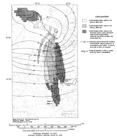
FIGURE 5.1 Contributing areas of wells and ponds in the complex flow system determined by using the three-dimensional model with 1987 average daily pumping rates. (Barlow 1993)
such as maximum prolonged pumping, prevail, and, therefore, conservatively large zones of contribution continue to be used for wellhead protection.
The ground water management experience of Cape Cod has resulted in a better understanding of the resource and the complexity of the aquifer
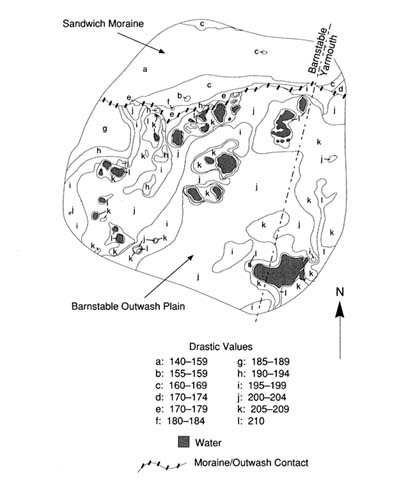
FIGURE 5.2 DRASTIC contours for Zone 1, Barnstable-Yarmouth, Massachusetts.
system, as well as the development of a more ambitious agenda for resource protection. Beginning with goals of protection of existing public water supplies, management interests have grown to include the protection of private wells, potential public supplies, fresh water ponds, and marine embayments. Public concerns over ground water quality have remained high and were a major factor in the creation of the Cape Cod Commission by the Massachusetts legislature. The commission is a land use planning and regulatory agency with broad authority over development projects and the ability to create special resource management areas. The net result of 20 years of effort by many individuals and agencies is the application of
TABLE 5.1 Ranges, Rating, and Weights for DRASTIC Study of Barnstable Outwash Plain Setting (NOTE: gpd/ft 2 = gallons per day per square foot) (Heath 1988)
| Factor | Range | Rating | Weight | Number |
| Depth to Water | 0-50+ feet | 5-10 | 5 | 25-50 |
| Net Recharge Per Year | 10+ inches | 9 | 4 | 36 |
| Aquifer Media | Sand & Gravel | 9 | 3 | 27 |
| Soil Media | Sand | 9 | 2 | 18 |
| Topography | 2-6% | 9 | 1 | 9 |
| Impact of Vadose Zone | Sand & Gravel | 8 | 5 | 40 |
| Hydraulic Conductivity | 2000+ gpd/ft | 10 | 3 | 30 |
|
|
|
|
| Total = 185-210 |
TABLE 5.2 Ranges, Rating, and Weights for DRASTIC Study of Sandwich Moraine Setting (NOTE: gpd/ft 2 = gallons per day per square foot) (Heath 1988)
| Factor | Range | Rating | Weight | Number |
| Depth to Water | 0-100+ feet | 1-10 | 5 | 5-50 |
| Net Recharge Per Year | 10+ inches | 9 | 4 | 36 |
| Aquifer Media | Sand & Gravel | 8 | 3 | 24 |
| Soil Media | Sandy Loam | 6 | 2 | 12 |
| Topography | 6-12% | 5 | 1 | 5 |
| Impact of Vadose Zone | Sand & Gravel | 8 | 5 | 40 |
| Hydraulic Conductivity | 700-1000 gpd/ft | 6 | 3 | 18 |
|
|
|
|
| Total = 140-185 |
higher protection standards to broader areas of the Cape Cod aquifer. With some exceptions for already impaired areas, a differentiated resource protection approach in the vulnerable aquifer setting of Cape Cod has resulted in a program that approaches universal ground water protection.
Florida has 13 million residents and is the fourth most populous state (U.S. Bureau of the Census 1991). Like several other sunbelt states, Florida's population is growing steadily, at about 1,000 persons per day, and is estimated to reach 17 million by the year 2000. Tourism is the biggest industry in Florida, attracting nearly 40 million visitors each year. Ground water is the source of drinking water for about 95 percent of Florida's population; total withdrawals amount to about 1.5 billion gallons per day. An additional 3 billion gallons of ground water per day are pumped to meet the needs of agriculture—a $5 billion per year industry, second only to tourism in the state. Of the 50 states, Florida ranks eighth in withdrawal of fresh ground water for all purposes, second for public supply, first for rural domestic and livestock use, third for industrial/commercial use, and ninth for irrigation withdrawals.
Most areas in Florida have abundant ground water of good quality, but the major aquifers are vulnerable to contamination from a variety of land use activities. Overpumping of ground water to meet the growing demands of the urban centers, which accounts for about 80 percent of the state's population, contributes to salt water intrusion in coastal areas. This overpumping is considered the most significant problem for degradation of ground water quality in the state. Other major sources of ground water contaminants include: (1) pesticides and fertilizers (about 2 million tons/year) used in agriculture, (2) about 2 million on-site septic tanks, (3) more than 20,000 recharge wells used for disposing of stormwater, treated domestic wastewater, and cooling water, (4) nearly 6,000 surface impoundments, averaging one per 30 square kilometers, and (5) phosphate mining activities that are estimated to disturb about 3,000 hectares each year.
The Hydrogeologic Setting
The entire state is in the Coastal Plain physiographic province, which has generally low relief. Much of the state is underlain by the Floridan aquifer system, largely a limestone and dolomite aquifer that is found in both confined and unconfined conditions. The Floridan is overlain through most of the state by an intermediate aquifer system, consisting of predominantly clays and sands, and a surficial aquifer system, consisting of predominantly sands, limestone, and dolomite. The Floridan is one of the most productive aquifers in the world and is the most important source of drinking water for Florida residents. The Biscayne, an unconfined, shallow, limestone aquifer located in southeast Florida, is the most intensively used
aquifer and the sole source of drinking water for nearly 3 million residents in the Miami-Palm Beach coastal area. Other surficial aquifers in southern Florida and in the western panhandle region also serve as sources of ground water.
Aquifers in Florida are overlain by layers of sand, clay, marl, and limestone whose thickness may vary considerably. For example, the thickness of layers above the Floridan aquifer range from a few meters in parts of west-central and northern Florida to several hundred meters in south-central Florida and in the extreme western panhandle of the state. Four major groups of soils (designated as soil orders under the U.S. Soil Taxonomy) occur extensively in Florida. Soils in the western highlands are dominated by well-drained sandy and loamy soils and by sandy soils with loamy subsoils; these are classified as Ultisols and Entisols. In the central ridge of the Florida peninsula, are found deep, well-drained, sandy soils (Entisols) as well as sandy soils underlain by loamy subsoils or phosphatic limestone (Alfisols and Ultisols). Poorly drained sandy soils with organic-rich and clay-rich subsoils, classified as Spodosols, occur in the Florida flatwoods. Organic-rich muck soils (Histosols) underlain by muck or limestone are found primarily in an area extending south of Lake Okeechobee.
Rainfall is the primary source of ground water in Florida. Annual rainfall in the state ranges from 100 to 160 cm/year, averaging 125 cm/year, with considerable spatial (both local and regional) and seasonal variations in rainfall amounts and patterns. Evapotranspiration (ET) represents the largest loss of water; ET ranges from about 70 to 130 cm/year, accounting for between 50 and 100 percent of the average annual rainfall. Surface runoff and ground water discharge to streams averages about 30 cm/year. Annual recharge to surficial aquifers ranges from near zero in perennially wet, lowland areas to as much as 50 cm/year in well-drained areas; however, only a fraction of this water recharges the underlying Floridan aquifer. Estimates of recharge to the Floridan aquifer vary from less than 3 cm/year to more than 25 cm/year, depending on such factors as weather patterns (e.g., rainfall-ET balance), depth to water table, soil permeability, land use, and local hydrogeology.
Permeable soils, high net recharge rates, intensively managed irrigated agriculture, and growing demands from urban population centers all pose considerable threat of ground water contamination. Thus, protection of this valuable natural resource while not placing unreasonable constraints on agricultural production and urban development is the central focus of environmental regulation and growth management in Florida.
Along with California, Florida has played a leading role in the United
States in development and enforcement of state regulations for environmental protection. Detection in 1983 of aldicarb and ethylene dibromide, two nematocides used widely in Florida's citrus groves, crystallized the growing concerns over ground water contamination and the need to protect this vital natural resource. In 1983, the Florida legislature passed the Water Quality Assurance Act, and in 1984 adopted the State and Regional Planning Act. These and subsequent legislative actions provide the legal basis and guidance for the Ground Water Strategy developed by the Florida Department of Environmental Regulation (DER).
Ground water protection programs in Florida are implemented at federal, state, regional, and local levels and involve both regulatory and nonregulatory approaches. The most significant nonregulatory effort involves more than 30 ground water studies being conducted in collaboration with the Water Resources Division of the U.S. Geological Survey. At the state level, Florida statutes and administrative codes form the basis for regulatory actions. Although DER is the primary agency responsible for rules and statutes designed to protect ground water, the following state agencies participate to varying degrees in their implementation: five water management districts, the Florida Geological Survey, the Department of Health and Rehabilitative Services (HRS), the Department of Natural Resources, and the Florida Department of Agriculture and Consumer Services (DACS). In addition, certain interagency committees help coordinate the development and implementation of environmental codes in the state. A prominent example is the Pesticide Review Council which offers guidance to the DACS in developing pesticide use regulation. A method for screening pesticides in terms of their chronic toxicity and environmental behavior has been developed through collaborative efforts of the DACS, the DER, and the HRS (Britt et al. 1992). This method will be used to grant registration for pesticide use in Florida or to seek additional site-specific field data.
Selecting an Approach
The emphasis of the DER ground water program has shifted in recent years from primarily enforcement activity to a technically based, quantifiable, planned approach for resource protection.
The administrative philosophy for ground water protection programs in Florida is guided by the following principles:
Ground water is a renewable resource, necessitating a balance between withdrawals and natural or artificial recharge.
Ground water contamination should be prevented to the maximum degree possible because cleanup of contaminated aquifers is technically or economically infeasible.
It is impractical, perhaps unnecessary, to require nondegradation standards for all ground water in all locations and at all times.
The principle of ''most beneficial use" is to be used in classifying ground water into four classes on the basis of present quality, with the goal of attaining the highest level protection of potable water supplies (Class I aquifers).
Part of the 1983 Water Quality Assurance Act requires Florida DER to "establish a ground water quality monitoring network designed to detect and predict contamination of the State's ground water resources" via collaborative efforts with other state and federal agencies. The three basic goals of the ground water quality monitoring program are to:
Establish the baseline water quality of major aquifer systems in the state,
Detect and predict changes in ground water quality resulting from the effects of various land use activities and potential sources of contamination, and
Disseminate to local governments and the public, water quality data generated by the network.
The ground water monitoring network established by DER to meet the goals stated above consists of two major subnetworks and one survey (Maddox and Spicola 1991). Approximately 1,700 wells that tap all major potable aquifers in the state form the Background Network, which was designed to help define the background water quality. The Very Intensively Studied Area (VISA) network was established to monitor specific areas of the state considered highly vulnerable to contamination; predominant land use and hydrogeology were the primary attributes used to evaluate vulnerability. The DRASTIC index, developed by EPA, served as the basis for statewide maps depicting ground water vulnerability. Data from the VISA wells will be compared to like parameters sampled from Background Network wells in the same aquifer segment. The final element of the monitoring network is the Private Well Survey, in which up to 70 private wells per county will be sampled. The sampling frequency and chemical parameters to be monitored at each site are based on several factors, including network well classification, land use activities, hydrogeologic sensitivity, and funding. In Figure 5.3 , the principal aquifers in Florida are shown along with the distribution of the locations of the monitoring wells in the Florida DER network.
The Preservation 2000 Act, enacted in 1990, mandated that the Land Acquisition Advisory Council (LAAC) "provide for assessing the importance
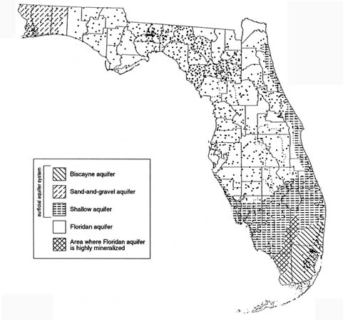
FIGURE 5.3 Principal aquifers in Florida and the network of sample wells as of March 1990 (1642 wells sampled). (Adapted from Maddox and Spicola 1991, and Maddox et al. 1993.)
of acquiring lands which can serve to protect or recharge ground water, and the degree to which state land acquisition programs should focus on purchasing such land." The Ground Water Resources Committee, a subcommittee of the LAAC, produced a map depicting areas of ground water significance at regional scale (1:500,000) (see Figure 5.4 ) to give decision makers the basis for considering ground water as a factor in land acquisition under the Preservation 2000 Act (LAAC 1991). In developing maps for their districts, each of the five water management districts (WMDs) used the following criteria: ground water recharge, ground water quality, aquifer vulnerability, ground water availability, influence of existing uses on the resource, and ground water supply. The specific approaches used by
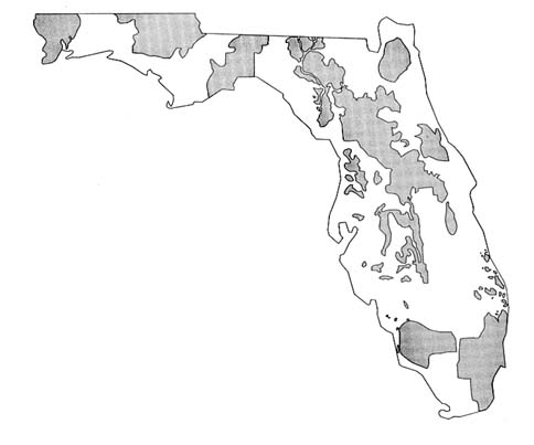
FIGURE 5.4 General areas of ground water significance in Florida. (Map provided by Florida Department of Environmental Regulation, Bureau of Drinking Water and Ground Water Resources.)
the WMDs varied, however. For example, the St. Johns River WMD used a GIS-based map overlay and DRASTIC-like numerical index approach that rated the following attributes: recharge, transmissivity, water quality, thickness of potable water, potential water expansion areas, and spring flow capture zones. The Southwest Florida WMD also used a map overlay and index approach which considered four criteria, and GIS tools for mapping. Existing databases were considered inadequate to generate a DRASTIC map for the Suwannee River WMD, but the map produced using an overlay approach was considered to be similar to DRASTIC maps in providing a general depiction of aquifer vulnerability.
In the November 1988, Florida voters approved an amendment to the Florida Constitution allowing land producing high recharge to Florida's aquifers to be classified and assessed for ad valorem tax purposes based on character or use. Such recharge areas are expected to be located primarily in the upland, sandy ridge areas. The Bluebelt Commission appointed by the 1989 Florida Legislature, studied the complex issues involved and recommended that the tax incentive be offered to owners of such high recharge areas if their land is left undeveloped (SFWMD 1991). The land eligible
for classification as "high water recharge land" must meet the following criteria established by the commission:
The parcel must be located in the high recharge areas designated on maps supplied by each of the five WMDs.
The high recharge area of the parcel must be at least 10 acres.
The land use must be vacant or single-family residential.
The parcel must not be receiving any other special assessment, such as Greenbelt classification for agricultural lands.
Two bills related to the implementation of the Bluebelt program are being considered by the 1993 Florida legislation.
THE SAN JOAQUIN VALLEY
Pesticide contamination of ground water resources is a serious concern in California's San Joaquin Valley (SJV). Contamination of the area's aquifer system has resulted from a combination of natural geologic conditions and human intervention in exploiting the SJV's natural resources. The SJV is now the principal target of extensive ground water monitoring activities in the state.
Agriculture has imposed major environmental stresses on the SJV. Natural wetlands have been drained and the land reclaimed for agricultural purposes. Canal systems convey water from the northern, wetter parts of the state to the south, where it is used for irrigation and reclamation projects. Tens of thousands of wells tap the sole source aquifer system to supply water for domestic consumption and crop irrigation. Cities and towns have sprouted throughout the region and supply the human resources necessary to support the agriculture and petroleum industries.
Agriculture is the principal industry in California. With 1989 cash receipts of more than $17.6 billion, the state's agricultural industry produced more than 50 percent of the nation's fruits, nuts, and vegetables on 3 percent of the nation's farmland. California agriculture is a diversified industry that produces more than 250 crop and livestock commodities, most of which can be found in the SJV.
Fresno County, the largest agricultural county in the state, is situated in the heart of the SJV, between the San Joaquin River to the north and the Kings River on the south. Grapes, stone fruits, and citrus are important commodities in the region. These and many other commodities important to the region are susceptible to nematodes which thrive in the county's coarse-textured soils.
While agricultural diversity is a sound economic practice, it stimulates the growth of a broad range of pest complexes, which in turn dictates greater reliance on agricultural chemicals to minimize crop losses to pests, and maintain productivity and profit. Domestic and foreign markets demand high-quality and cosmetically appealing produce, which require pesticide use strategies that rely on pest exclusion and eradication rather than pest management.
Hydrogeologic Setting
The San Joaquin Valley (SJV) is at the southern end of California's Central Valley. With its northern boundary just south of Sacramento, the Valley extends in a southeasterly direction about 400 kilometers (250 miles) into Kern County. The SJV averages 100 kilometers (60 miles) in width and drains the area between the Sierra Nevada on the east and the California Coastal Range on the west. The rain shadow caused by the Coastal Range results in the predominantly xeric habitat covering the greater part of the valley floor where the annual rainfall is about 25 centimeters (10 inches). The San Joaquin River is the principal waterway that drains the SJV northward into the Sacramento Delta region.
The soils of the SJV vary significantly. On the west side of the valley, soils are composed largely of sedimentary materials derived from the Coastal Range; they are generally fine-textured and slow to drain. The arable soils of the east side developed on relatively unweathered, granitic sediments. Many of these soils are wind-deposited sands underlain by deep coarse-textured alluvial materials.
From the mid-1950s until 1977, dibromochloropropane (DBCP) was the primary chemical used to control nematodes. DBCP has desirable characteristics for a nematocide. It is less volatile than many other soil fumigants, such as methylbromide; remains active in the soil for a long time, and is effective in killing nematodes. However, it also causes sterility in human males, is relatively mobile in soil, and is persistent. Because of the health risks associated with consumption of DBCP treated foods, the nematocide was banned from use in the United States in 1979. After the ban, several well water studies were conducted in the SJV by state, county and local authorities. Thirteen years after DBCP was banned, contamination of well waters by the chemical persists as a problem in Fresno County.
Public concern over pesticides in ground water resulted in passage of the California Pesticide Contamination Prevention Act (PCPA) of 1985. It is a broad law that establishes the California Department of Pesticide Regulation
as the lead agency in dealing with issues of ground water contamination by pesticides. The PCPA specifically requires:
pesticide registrants to collect and submit specific chemical and environmental fate data (e.g., water solubility, vapor pressure, octanol-water partition coefficient, soil sorption coefficient, degradation half-lives for aerobic and anaerobic metabolism, Henry's Law constant, hydrolysis rate constant) as part of the terms for registration and continued use of their products in California.
establishment of numerical criteria or standards for physical-chemical characteristics and environmental fate data to determine whether a pesticide can be registered in the state that are at least as stringent as those standards set by the EPA,
soil and water monitoring investigations be conducted on:
pesticides with properties that are in violation of the physical-chemical standards set in 2 above, and
pesticides, toxic degradation products or other ingredients that are:
contaminants of the state's ground waters, or
found at the deepest of the following soil depths:
2.7 meters (8 feet) below the soil surface,
below the crop root zone, or
below the microbial zone, and
creation of a database of wells sampled for pesticides with a provision requiring all agencies to submit data to the California Department of Pesticide Regulation (CDPR).
Difficulties associated with identifying the maximum depths of root zone and microbial zone have led to the establishment of 8 feet as a somewhat arbitrary but enforceable criterion for pesticide leaching in soils.
Selection and Implementation of an Approach
Assessment of ground water vulnerability to pesticides in California is a mechanical rather than a scientific process. Its primary goal is compliance with the mandates established in the PCPA. One of these mandates requires that monitoring studies be conducted in areas of the state where the contaminant pesticide is used, in other areas exhibiting high risk portraits (e.g., low organic carbon, slow soil hydrolysis, metabolism, or dissipation), and in areas where pesticide use practices present a risk to the state's ground water resources.
The numerical value for assessments was predetermined by the Pesticide Use Report (PUR) system employed in the state. Since the early
1970s, California has required pesticide applicators to give local authorities information on the use of restricted pesticides. This requirement was extended to all pesticides beginning in 1990. Application information reported includes names of the pesticide(s) and commodities, the amount applied, the formulation used, and the location of the commodity to the nearest section (approximately 1 square mile) as defined by the U.S. Rectangular Coordinate System. In contrast to most other states that rely on county pesticide sales in estimating pesticide use, California can track pesticide use based on quantities applied to each section. Thus, the section, already established as a political management unit, became the basic assessment unit.
The primary criteria that subject a pesticide to investigation as a ground water pollutant are:
detection of the pesticide or its metabolites in well samples, or
its failure to conform to the physical-chemical standards set in accordance with the PCPA, hence securing its position on the PCPA's Ground Water Protection List of pesticides having a potential to pollute ground water.
In either case, relatively large areas surrounding the original detection site or, in the latter case, high use regions are monitored via well surveys. Positive findings automatically increase the scope of the surveys, and since no tolerance levels are specified in the PCPA, any detectable and confirmed result establishes a pesticide as a contaminant.
When a pesticide or its degradation products is detected in a well water sample and the pesticide is judged to have contaminated the water source as a result of a legal agricultural use, the section the well is in is declared a Pesticide Management Zone (PMZ). Further application of the detected pesticide within PMZ boundaries may be prohibited or restricted, depending on the degree of contamination and subject to the availability of tried and tested modifications in management practices addressing environmental safety in use of the pesticide. PMZs are pesticide-specific—each contaminant pesticide has its own set of PMZs which may or may not overlap PMZs assigned another pesticide. Currently, consideration is being given to the extension of PMZs established for one chemical to other potential pesticide pollutants. In addition to monitoring activities in PMZs, protocols have been written to monitor ground water in sections adjacent to a PMZ. Monitoring of adjacent sections has resulted in many new PMZs. Currently, California has 182 PMZs involving five registered pesticides.
California has pursued this mechanical approach to assessing ground water vulnerability to pesticides for reasons that cover a spectrum of political, economic, and practical concerns. As noted earlier, the scale of the assessment unit was set at the section level because it is a well-defined
geopolitical unit used in the PUR system. Section boundaries frequently are marked by roads and highways, which allows the section to be located readily and makes enforcement of laws and regulations more practical. California law also requires that well logs be recorded by drillers for all wells in the state. Well-site information conforms to the U.S. Rectangular Coordinate System's township, range, and section system.
The suitability and reliability of databases available for producing vulnerability assessments was a great concern before passage of the PCPA in 1985. Soil survey information holds distinct advantages for producing assessments and developing best management practices strategies, but it was not available in a format that could work in harmony with PUR sections. To date, several areas of the SJV are not covered by a modern soil survey; they include the western part of Tulare County, which contains 34 PMZs. Other vadose zone data were sparse, it available at all.
The use of models was not considered appropriate, given the available data and because no single model could cope with the circumstances in which contaminated ground water sources were being discovered in the state. While most cases of well contamination were associated with the coarse-textured soils of the SJV and the Los Angeles Basin, several cases were noted in areas of the Central Valley north of the SJV, where very dense fine-textured soils (vertisols and other cracking clays) were dominant.
The potential vagaries and uncertainties associated with more scientific approaches to vulnerability assessment, given the tools available when the PCPA was enacted, presented too large a risk for managers to consider endorsing their use. In contrast, the basic definition of the PMZ is difficult to challenge (pesticide contamination has been detected or not detected) in the legal sense. And the logic of investing economic resources in areas immediately surrounding areas of acknowledged contamination are relatively undisputable. The eastern part of the SJV contains more than 50 percent of the PMZs in the state. Coarse-textured soils of low carbon content are ubiquitous in this area and are represented in more than 3,000 sections. The obvious contamination scenario is the normal scenario in the eastern SJV, and because of its size it creates a huge management problem. While more sophisticated methods for assessing ground water vulnerability have been developed, a question that begs to be asked is "How would conversion to the use of enhanced techniques for evaluating ground water vulnerability improve ground water protection policy and management in the SJV?"
More than 90 percent of the population of Hawaii depends on ground water (nearly 200 billion gallons per day) for their domestic supply (Au 1991). Ground water contamination is of special concern in Hawaii, as in other insular systems, where alternative fresh water resources are not readily available or economically practical. Salt water encroachment, caused by pumping, is by far the biggest source of ground water contamination in Hawaii; however, nonpoint source contamination from agricultural chemicals is increasingly a major concern. On Oahu, where approximately 80 percent of Hawaii's million-plus population resides, renewable ground water resources are almost totally exploited; therefore, management action to prevent contamination is essential.
Each of the major islands in the Hawaiian chain is formed from one or more shield volcanoes composed primarily of extremely permeable thin basaltic lava flows. On most of the Hawaiian islands the margins of the volcanic mountains are overlapped by coastal plain sediments of alluvial and marine origin that were deposited during periods of volcanic quiescence. In general, the occurrence of ground water in Hawaii, shown in Figure 5.5 , falls into three categories: (1) basal water bodies floating on and displacing salt water, (2) high-level water bodies impounded within compartments formed by impermeable dikes that intrude the lava flows, and (3) high-level water bodies perched on ash beds or soils interbedded with
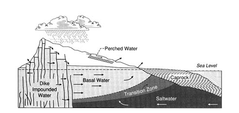
FIGURE 5.5 Cross section of a typical volcanic dome showing the occurrence of ground water in Hawaii (After Peterson 1972. Reprinted, by permission, from Water Well Journal Publishing Company, 1972.)
thin lava flows on unconformities or on other relatively impervious lava flows (Peterson 1972).
A foundation of the tourist industry in Hawaii is the pristine environment. The excellent quality of Hawaii's water is well known. The public has demanded, and regulatory agencies have adopted, a very conservative, zero-tolerance policy on ground water contamination. The reality, however, is that past, present, and future agricultural, industrial, and military activities present potentially significant ground water contamination problems in Hawaii.
Since 1977 when 1,874 liters of ethylene dibromide (EDB) where spilled within 18 meters of a well near Kunia on the island of Oahu, the occurrence and distribution of contaminants in Hawaii's ground water has been carefully documented by Oki and Giambelluca (1985, 1987) and Lau and Mink (1987). Before 1981, when the nematocide dibromochloropropane (DBCP) was found in wells in central Oahu, the detection limit for most chemicals was too high to reveal the low level of contamination that probably had existed for many years.
Concern about the fate of agriculture chemicals led the Hawaii State Department of Agriculture to initiate a large sampling program to characterize the sources of nonpoint ground water contamination. In July 1983, 10 wells in central Oahu were closed because of DBCP and EDB contamination. The public has been kept well informed of possible problems through the publication of maps of chemicals detected in ground water in the local newspaper. Updated versions of these maps are shown in Figures 5.6a , b , c , and d .
In Hawaii, interagency committees, with representation from the Departments of Health and Agriculture, have been formed to address the complex technical and social questions associated with ground water contamination from agricultural chemicals. The Hawaii legislature has provided substantial funding to groups at the University of Hawaii to develop the first GIS-based regional scale chemical leaching assessment approach to aid in pesticide regulation. This effort, described below, has worked to identify geographic areas of concern, but the role the vulnerability maps generated by this system will play in the overall regulatory process is still unclear.
Agrichemicals are essential to agriculture in Hawaii. It is not possible to maintain a large pineapple monoculture in Hawaii without nematode control using pesticides. Pineapple and sugar growers in Hawaii have generally employed well controlled management practices in their use of fertilizers, herbicides, and insecticides. In the early 1950s, it was thought that organic chemicals such as DBCP and EDB would not leach to ground water
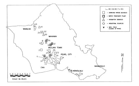
FIGURE 5.6a The occurrence and distribution of ground water contamination on the Island of Oahu. (Map provided by Hawaii State Department of Health.)
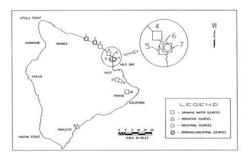
FIGURE 5.6b The occurrence and distribution of ground water contamination on the Island of Hawaii. (Map provided by Hawaii State Department of Health.)
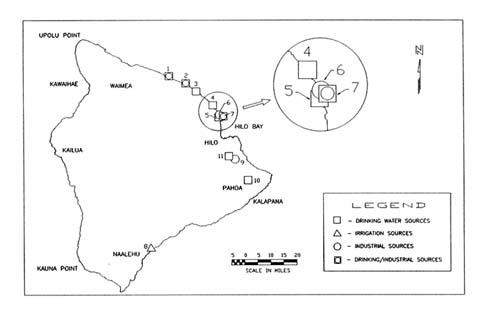
FIGURE 5.6c The occurrence and distribution of ground water contamination on the Island of Maui. (Map provided by Hawaii State Department of Health.)
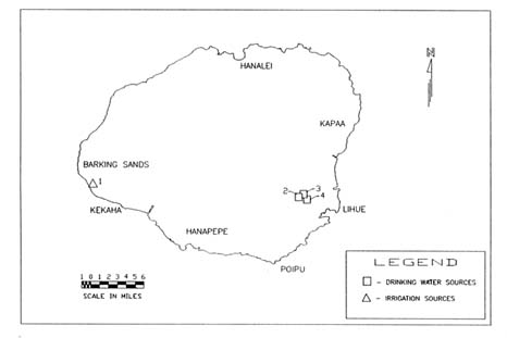
FIGURE 5.6d The occurrence and distribution of ground water contamination on the Island of Kauai. (Map provided by Hawaii State Department of Health.)
because (1) the chemicals are highly sorbed in soils with high organic carbon contents, (2) the chemicals are highly volatile, and (3) the water table is several hundred meters below the surface. Measured concentrations of DBCP and EDB down to 30 meters at several locations have shown the original assessment to be wrong. They have resulted in an urgent need to understand processes such as preferential flow better and to predict if the replacement chemicals used today, such as Telon II, will also leach to significant depths.
Leaching of pesticides to ground water in Hawaii could take decades. This time lag could lead to a temporary false sense of security, as happened in the past and potentially result in staggering costs for remedial action. For this reason, mathematical models that permit the user to ask ''what if" questions have been developed to help understand what the future may hold under certain management options. One needs to know what the fate of chemicals applied in the past will be and how to regulate the chemicals considered for use in the future; models are now being developed and used to help make these vulnerability assessments.
Researchers have embarked on several parallel approaches to quantitatively assess the vulnerability of Hawaii's ground water resources, including: (1) sampling, (2) physically-based numerical modeling, and (3) vulnerability mapping based on a simple chemical leaching index. Taken together these approaches have provided insight and guidance for work on a complex, spatially and temporally variable problem.
The sampling programs (Wong 1983 and 1987, Peterson et al. 1985) have shown that the chemicals applied in the past do, in fact, leach below the root zone, contrary to the original predictions, and can eventually reach the ground water. Experiments designed to characterize the nuances of various processes, such as volatilization, sorption, and degradation, have been conducted recently and will improve the conceptualization of mathematical models in the future.
The EPA's Pesticide Root Zone Model (PRZM), a deterministic-empirical/conceptual fluid flow/solute transport model, has been tested by Loague and co-workers (Loague et al. 1989a, b; Loague 1992) against measured concentration profiles for DBCP and EDB in central Oahu. These simulations illustrate that the chemicals used in the past can indeed move to considerable depths. Models of this kind, once properly validated, can be used to simulate the predicted fate of future pesticide applications. One must always remember, however, that numerical simulations must be interpreted in terms of the limiting assumptions associated with model and data errors.
Ground water vulnerability maps and assessments of their uncertainty were pioneered at the University of Hawaii in the Department of Agriculture Engineering (Khan and Liang 1989, Loague and Green 1990a). These pesticide leaching assessments were made by coupling a simple mobility index to a geographic information system. Loague and coworkers have investigated the uncertainty in these maps owing to data and model errors (Loague and Green 1988; Loague et al. 1989c, 1990; Loague and Green 1990b, 1990c; Loague 1991; Kleveno et al. 1992; Yost et al. 1993). The Hawaiian database on soils, climate, and chemicals is neither perfect nor poor for modeling applications; it is typical of what exists in most states—major extrapolations are required to estimate the input parameters required for almost any chemical fate model.
Sampling from wells in Hawaii has shown the concentrations of various chemicals, both from agriculture and industrial sources, which have leached to ground water in Hawaii. These concentrations, in general, are low compared to the levels detected in other states and for the most part are below health advisory levels established by EPA. In some instances contamination has not resulted from agriculture, but rather from point sources such as chemical loading and mixing areas and possibly from ruptured fuel lines. The widespread presence of trichloropropane (TCP) in Hawaii's ground water and deep soil cores at concentrations higher than DBCP was totally unexpected. TCP was never applied as a pesticide, but results from the manufacture of the fumigant DD, which was used until 1977 in pineapple culture. The occurrence of TCP illustrates that one must be aware of the chemicals applied as well as their components and transformation products.
Wells have been closed in Hawaii even though the measured contaminant concentrations have been below those considered to pose a significant health risk. At municipal well locations in central Oahu, where DBCP, EDB, and/or TCP have been detected, the water is now passed through carbon filters before it is put into the distribution system. The cost of this treatment is passed on to the water users, rather than to those who applied the chemicals.
The pesticide leaching assessment maps developed by Khan and Liang (1989) are intended for incorporation into the regulatory process. Decisions are not made on the basis of the red and green shaded areas for different chemicals (see Plate 3 ), but this information is considered. The uncertainty analysis by Loague and coworkers has shown some of the limitations of deterministic assessments in the form of vulnerability maps and provided initial guidance on data shortfalls.
APPLICATION OF A VULNERABILITY INDEX FOR DECISION-MAKING AT THE NATIONAL LEVEL
Need for a vulnerability index.
A vulnerability index for ground water contamination by pesticides has been developed and used by USDA as a decision aid to help attain the objectives of the President's Water Quality Initiative (see Box 1.1 ). A vulnerability index was needed for use in program management and to provide insight for policy development. Motivation for the development of the vulnerability index was provided by two specific questions:
Given limited resources and the geographic diversity of the water quality problems associated with agricultural production, what areas of the country have the highest priority for study and program implementation?
What policy implications emerge from the spatial patterns of the potential for conamination from a national perspective, given information currently available about farming practices and chemical use in agriculture?
Description of the Vulnerability Index
A vulnerability index was derived to evaluate the likelihood of shallow ground water contamination by pesticides used in agriculture in one area compared to another area. Because of the orientation of Initiative policies to farm management practices, it was necessary that the vulnerability measure incorporate field level information on climate, soils, and chemical use. It also needed to be general enough to include all areas of the country and all types of crops grown.
A Ground Water Vulnerability Index for Pesticides (GWVIP) was developed by applying the Soil-Pesticide Interaction Screening Procedure (SPISP) developed by the Soil Conservation Service to the National Resource Inventory (NRI) land use database for 1982 and the state level pesticide use database created by Resources for the Future (Gianessi and Puffer 1991). Details of the computational scheme and databases used are described by Kellogg et al. (1992). The 1982 NRI and the associated SOIL-5 database provide information on soil properties and land use at about 800,000 sample points throughout the continental United States. This information is sufficient to apply the SPISP to each point and thus obtain a relative measure of the soil leaching potential throughout the country. The RFF pesticide use database was used to infer chemical use at each point on the basis of the crop type recorded in the NRI database. By taking advantage of the statistical properties of the NRI database, which is based on a statistical survey
sampling design, the GWVIP score at each of the sample points can be statistically aggregated for making comparisons among regions.
Since the GWVIP is an extension of a screening procedure, it is designed to minimize the likelihood of incorrectly identifying an area as having a low potential for contamination—that is, false negatives are minimized and false positives are tolerated. The GWVIP is designed to classify an area as having a potential problem even if the likelihood is small.
GWVIP scores were graphically displayed after embedding them in a national cartographic database consisting of 13,172 polygons created by overlaying the boundaries of 3,041 counties, 189 Major Land Resource Areas (MLRAs), 2,111 hydrologic units, and federal lands.
Three caveats are especially important in using the GWVIP and its aggregates as a decision aid:
Land use data are for 1982 and do not represent current cropping patterns in some parts of the country. Although total cropland acreage has remained fairly stable over the past 10 years, there has been a pronounced shift from harvested cropland to cropland idled in government programs.
The approach uses a simulation model that predicts the amount of chemical that leaches past the root zone. In areas where the water table is near the surface, these predictions relate directly to shallow ground water contamination. In other areas a time lag is involved. No adjustment was made for areas with deep water tables.
No adjustment in chemical use is made to account for farm management factors, such as chemical application rates and crop rotations. The approach assumes that chemical use is the same for a crop grown as part of a rotation cropping system as for continuous cropping. Since the chemical use variable in the GWVIP calculation is based on acres of land treated with pesticides, application rates are also not factored into the analysis.
Application to Program Management
By identifying areas of the country that have the highest potential for leaching of agrichemicals, the GWVIP can serve as a basis for selecting sites for implementation of government programs and for more in-depth research on the environmental impact of agrichemical use. These sites cannot be selected exclusively on the basis of the GWVIP score, however, because other factors, such as surface water impacts and economic and demographic factors, are also important.
For example, the GWVIP has been used as a decision aid in selecting sites for USDA's Area Study Program, which is designed to provide chemical use and farming practice information to aid in understanding the relationships among farming activities, soil properties, and ground water quality.
The National Agricultural Statistics Service interviews farm operators in 12 major watersheds where the U.S. Geological Survey is working to measure the quality of surface and ground water resources under its National Water Quality Assessment Program. At the conclusion of the project, survey information will be combined with what is learned in other elements of the President's Water Quality Initiative to assess the magnitude of the agriculture-related water quality problem for the nation as a whole and used to evaluate the potential economic and environmental effects of Initiative policies of education, technical assistance, and financial assistance if implemented nationwide.
To meet these objectives, each Area Study site must have a high potential for ground water contamination relative to other areas of the country. A map showing the average GWVIP for each of the 13,172 polygons comprising the continental United States, shown in Plate 3 , was used to help select the sites. As this map shows, areas more likely to have leaching problems with agrichemicals than other areas of the country occur principally along the coastal plains stretching from Alabama and Georgia north to the Chesapeake Bay area, the corn belt states, the Mississippi River Valley, and the irrigated areas in the West. Sites selected for study in 1991 and 1992 include four from the eastern coastal plain (Delmarva Peninsula, southeastern Pennsylvania, Virginia and North Carolina, and southern Georgia), four from the corn belt states (Nebraska, Iowa, Illinois, and Indiana), and two from the irrigated areas in the West (eastern Washington and southeastern Idaho). Four additional sites will be selected for study in 1993.
Application to Policy Analysis and Development
The GWVIP has also been used by USDA to provide a national perspective on agricultural use of pesticides and the potential for ground water contamination to aid in policy analysis and development.
The geographic distribution of GWVIP scores has shown that the potential for ground water contamination is diverse both nationally and regionally. Factors that determine intrinsic vulnerability differ in virtually every major agricultural region of the country. Whether an impact is realized in these intrinsically vulnerable areas depends on the activities of producers—such as the type of crop planted, chemical use, and irrigation practices—which also vary both nationally and regionally. High vulnerability areas are those where a confluence of these factors is present. But not all cropland is vulnerable to leaching. About one-fourth of all cropland has GWVIP scores that indicate very low potential for ground water contamination from the use of agrichemicals. Nearly all agricultural states have significant acreage that meets this low vulnerability criterion. Areas of the country identified as being in a high vulnerability group relative to potential
for agrichemical leaching also have significant acreages that appear to have low vulnerability.
This mix of relative vulnerabilities both nationally and regionally has important policy implications. With the potential problem so diverse, it is not likely that simple, across-the-board solutions will work. Simple policies—such as selective banning of chemicals—may reduce the potential for ground water contamination in problem areas while imposing unnecessary costs on farming in nonproblem areas. The geographic diversity of the GWVIP suggests that the best solutions will come from involvement of both local governments and scientists with their state and national counter-parts to derive policies that are tailored to the unique features of each problem area.
In the future, USDA plans to use vulnerability indexes, like the GWVIP, in conjunction with economic models to evaluate the potential for solving agriculture-related water quality problems with a nationwide program to provide farmers with the knowledge and technical means to respond voluntarily to water quality concerns.
These six case studies illustrate how different approaches to vulnerability assessment have evolved under diverse sets of management requirements, data constraints, and other technical considerations. In addition, each of these examples shows that vulnerability assessment is an ongoing process through which information about a region's ground water resources and its quality can be organized and examined methodically.
In Iowa, the Iowa DNR staff elected to keep their vulnerability characterization efforts as simple as possible, and to use only properties for which data already existed or could be easily checked. They assumed that surficial features such as the soil are too thin and too disrupted by human activities (e.g., tillage, abandoned wells) to provide effective ground water protection at any particular location and sought to identify a surrogate measure for average travel time from the land surface to the aquifer. Thus, a ground water vulnerability map was produced which represents vulnerability primarily on the basis of depth to ground water and extent of overlying materials. Wells and sinkholes are also shown. The results are to be used for informing resource managers and the public of the vulnerability of the resource and to determine the type of information most needed to develop an even better understanding of the vulnerability of Iowa's ground water.
The Cape Cod approach to ground water vulnerability assessment is perhaps one of the oldest and most sophisticated in the United States. Driven by the need to protect the sole source drinking water aquifer underlying this sandy peninsula, the vulnerability assessment effort has focused on the identification
and delineation of the primary recharge areas for the major aquifers. This effort began with a simple mass balance approach which assumed even recharge within a circular area around each drinking water well. It has since evolved to the development of a complex, particle-tracking three-dimensional model that uses site-specific data to delineate zones of contribution. Bolstered by strong public concern, Cape Cod has been able to pursue an ambitious and sophisticated agenda for resource protection, and now boasts a sophisticated differential management ground water protection program.
In Florida, ground water resource managers rely on a combination of monitoring and vulnerability assessment techniques to identify high recharge areas the develop the state ground water protection program. Overlay and index methods, including several modified DRASTIC maps were produced to identify areas of ground water significance in support of decision making in state land acquisition programs aimed at ground water protection. In addition, several monitoring networks have been established to assess background water quality and monitor actual effects in areas identified as highly vulnerable. The coupling of ground water vulnerability assessments with monitoring and research efforts, provides the basis of an incremental and evolving ground water protection program in Florida.
The programs to protect ground water in California's intensely agricultural San Joaquin Valley are driven largely by compliance with the state Pesticide Contamination Prevention Act. The California Department of Pesticide Regulation determined that no model would be sufficient to cover their specific regulatory needs and that the available data bases were neither suitable nor reliable for regulatory purposes. Thus, a ground water protection program was built on the extensive existing pesticide use reporting system and the significant ground water monitoring requirements of the act. Using farm sections as management units, the state declares any section in which a pesticide or its degradation product is detected as a pesticide management zone and establishes further restrictions and monitoring requirements. Thus, the need to devise a defensible regulatory approach led California to pursue a mechanistic monitoring based approach rather than a modeling approach that would have inherent and difficult to quantify uncertainties.
In contrast, the approach taken in Hawaii involves an extensive effort to understand the uncertainty associated with the assessment models used. The purpose of this is to provide guidance to, but not the sole basis for, the pesticide regulation program. The combined use of sampling, physically-based numerical modeling, and a chemical leaching index has led to extensive improvements in the understanding of the fate of pesticides in the subsurface environment. Uncertainty analyses are used to determine where additional information would be most useful.
Finally, USDA's Ground Water Vulnerability Index for Pesticides illustrates a national scale vulnerability assessment developed for use as a decision aid and analytical tool for national policies regarding farm management and water quality. This approach combines nationally available statistical information on pesticide usage and soil properties with a simulation model to predict the relative likelihood of contamination in cropland areas. USDA has used this approach to target sites for its Area Study Program which is designed to provide information to farmers about the relationships between farm management practices and water quality. The results of the GWVIP have also indicated that, even at the regional level, there is often an mix of high and low vulnerability areas. This result suggests that effective ground water policies should be tailored to local conditions.
Au, L.K.L. 1991. The Relative Safety of Hawaii's Drinking Water. Hawaii Medical Journal 50(3): 71-80.
Barlow, P.M. 1993. Particle-Tracking Analysis of Contributing Areas of Public-Supply Wells in Simple and Complex Flow Systems, Cape Cod, Massachusetts. USGS Open File Report 93-159. Marlborough, Massachusetts: U.S. Geological Survey.
Britt, J.K., S.E. Dwinell, and T.C. McDowell. 1992. Matrix decision procedure to assess new pesticides based on relative ground water leaching potential and chronic toxicity. Environ. Toxicol. Chem. 11: 721-728.
Cape Cod Commission (CCC). 1991. Regional Policy Plan. Barnstable, Massachusetts: Cape Cod Commission.
Cape Cod Planning and Economic Development Commission (CCPEDC). March 1978a. Draft Area Wide Water Quality Management Plan for Cape Cod. Barnstable, Massachusetts: Cape Cod Commission.
Cape Cod Planning and Economic Development Commission (CCPEDC). September 1978b. Final Area Wide Water Quality Management Plan for Cape Cod. Barnstable, Massachusetts: Cape Cod Commission.
Department of Environmental Protection, Division of Water Supply (DEP-WS). 1991. Guidelines and Policies for Public Water Supply Systems. Massachusetts Department of Environmental Protection.
Gianessi, L.P., and C.A. Puffer. 1991. Herbicide Use in the United States: National Summary Report. Washington, D.C.: Resources for the Future.
Guswa, J.H., and D.R. LeBlanc. 1981. Digital Models of Ground water Flow in the Cape Cod Aquifer System, MA. USGS Water Supply Paper 2209. U.S. Geological Survey.
Heath, D.L. 1988. DRASTIC mapping of aquifer vulnerability in eastern Barnstable and western Yarmouth, Cape Cod, Massachusetts. In Appendix D, Cape Cod Aquifer Management Project, Final Report, G.A. Zoto and T. Gallagher, eds. Boston: Massachusetts Department of Environmental Quality Engineering.
Horsely, S.W. 1983. Delineating zones of contribution of public supply wells to protect ground water . In Proceedings of the National Water Well Association Eastern Regional Conference, Ground-Water Management, Orlando, Florida.
Hoyer, B.E. 1991. Ground water vulnerability map of Iowa. Pp. 13-15 in Iowa Geology, no. 16. Iowa City, Iowa: Iowa Department of Natural Resources.
Hoyer, B.E., J.E. Combs, R.D. Kelley, C. Cousins-Leatherman, and J.H. Seyb. 1987. Iowa Ground water Protection Strategy. Des Moines: Iowa Department of Natural Resources.
Kellogg, R.L., M.S. Maizel, and D.W. Goss. 1992. Agricultural Chemical Use and Ground Water Quality: Where Are the Potential Problems? Washington, D.C.: U.S. Department of Agriculture, Soil Conservation Service.
Khan, M.A., and T. Liang. 1989. Mapping pesticide contamination potential. Environmental Management 13(2):233-242.
Kleveno, J.J., K. Loague, and R.E. Green. 1992. An evaluation of a pesticide mobility index: Impact of recharge variation and soil profile heterogeneity. Journal of Contaminant Hydrology 11(1-2):83-99.
Land Acquisition Advisory Council (LAAC). 1991. Ground Water Resources Committee Final Report: Florida Preservation 2000 Needs Assessment. Tallahassee, Florida: Department of Environmental Regulation. 39 pp.
Lau, L.S., and J.F. Mink. 1987. Organic contamination of ground water: A learning experience. J. American Water Well Association 79(8):37-42.
LeBlanc, D.R., and J.H. Guswa. 1977. Water-Table Map of Cape Cod, MA. May 23-27, 1976, USGS Open File Report 77-419, scale 1:48,000.
Loague, K. 1991. The impact of land use on estimates of pesticide leaching potential: Assessments and uncertainties. Journal of Contaminant Hydrology 8: 157-175.
Loague, K. 1992. Simulation of organic chemical movement in Hawaii soils with PRZM: 3. Calibration. Pacific Science 46(3):353-373.
Loague, K.M., and R.E. Green. 1988. Impact of data-related uncertainties in a pesticide leaching assessment. Pp. 98-119 in Methods for Ground Water Quality Studies, D.W. Nelson and R.H. Dowdy, eds. Lincoln, Nebraska: Agricultural Research Division, University of Nebraska.
Loague, K., and R.E. Green. 1990a. Comments on "Mapping pesticide contamination potential," by M.A. Khan and T. Liang. Environmental Management 4:149-150.
Loague, K., and R.E. Green. 1990b. Uncertainty in Areal Estimates of Pesticide Leaching Potential. Pp. 62-67 in Transactions of 14th International Congress of Soil Science. Kyoto, Japan: International Soil Science Society.
Loague, K., and R.E. Green. 1990c. Criteria for evaluating pesticide leaching models. Pp. 175-207 in Field-Scale Water and Solute Flux in Soils, K. Roth, H. Flühler, W.A. Jury, and J.C. Parker, eds. Basel, Switzerland: Birkhauser Verlag.
Loague, K.M., R.E. Green, C.C.K. Liu, and T.C. Liang. 1989a. Simulation of organic chemical movement in Hawaii soils with PRZM: 1. Preliminary results for ethylene dibromide. Pacific Science 43(1):67-95.
Loague, K., T.W. Giambelluca, R.E. Green, C.C.K. Liu, T.C. Liang, and D.S. Oki. 1989b. Simulation of organic chemical movement in Hawaii soils with PRZM: 2. Predicting deep penetration of DBCP, EDB, and TCP. Pacific Science 43(4):362-383.
Loague, K.M., R.S. Yost, R.E. Green, and T.C. Liang. 1989c. Uncertainty in a pesticide leaching assessment for Hawaii. Journal of Contaminant Hydrology 4:139-161.
Loague, K., R.E. Green, T.W. Giambelluca, T.C. Liang, and R.S. Yost. 1990. Impact of uncertainty in soil, climatic, and chemical information in a pesticide leaching assessment. Journal of Contaminant Hydrology 5:171-194.
Maddox, G., and J. Spicola. 1991. Ground Water Quality Monitoring Network. Tallahassee, Florida: Florida Department of Environmental Regulation. 20 pp.
Maddox, G., J. Lloyd, T. Scott, S. Upchurch, and R. Copeland, eds. 1993. Florida's Ground Water Quality monitoring Program: Background Hydrogeochemistry. Florida Geological Survey Special Publication #34. Tallahassee, Florida: Florida Department of Environmental Regulation in cooperation with Florida Geological Survey.
National Research Council (NRC). 1986. Ground Water Quality Protection: State and Local Strategies. Washington, D.C.: National Academy Press.
Oki, D.S., and T.W. Giambelluca. 1985. Subsurface Water and Soil Quality Data Base for State of Hawaii: Part 1. Spec. Rept. 7. Manoa, Hawaii: Water Resources Research Center, University of Hawaii at Manoa.
Oki, D.S., and T.W. Giambelluca. 1987. DBCP, EDB, and TCP contamination of ground water in Hawaii. Ground Water 25:693-702.
Olimpio, J.C., E.C. Flynn, S. Tso, and P.A. Steeves. 1991. Use of a Geographic Information System to Assess Risk to Ground-Water Quality at Public-Supply Wells, Cape Cod, Massachusetts. Boston, Massachusetts: U.S. Geological Survey.
Peterson, F.L. 1972. Water development on tropic volcanic islands—Type example: Hawaii. Ground Water 5:18-23.
Peterson, F.L., K.R. Green, R.E. Green, and J.N. Ogata. 1985. Drilling program and pesticide analysis of core samples from pineapple fields in central Oahu. Water Resources Research Center, University of Hawaii at Manoa, Special Report 7.5. Photocopy.
Southwest Florida Water Management Districts (SFWMD). 1991. The Bluebelt Commission. Brooksville, Florida: Southwest Florida Water Management Districts.
U.S. Bureau of the Census. 1991. Statistical Abstracts of the United States: 1991, 111th edition. Washington, D.C.: U.S. Government Printing Office.
Wong, L. 1983. Preliminary report on soil sampling EDB on Oahu. Pesticide Branch, Div. of Plant Industry, Department of Agriculture, State of Hawaii. Photocopy.
Wong, L. 1987. Analysis of ethylene dibromide distribution in the soil profile following shank injection for nematode control in pineapple culture. Pp. 28-40 in Toxic Organic Chemicals in Hawaii's Water Resources, P.S.C. Rao and R.E. Green, eds. Ser. 086. Honolulu: Hawaii Inst. Trop Agric. Hum. Resources Res. Exten. University of Hawaii.
Yost, R.S., K. Loague, and R.E. Green. 1993. Reducing variance in soil organic carbon estimates—soil classification and geostatistical approaches. Geoderma 57(3):247-262
Since the need to protect ground water from pollution was recognized, researchers have made progress in understanding the vulnerability of ground water to contamination. Yet, there are substantial uncertainties in the vulnerability assessment methods now available.
With a wealth of detailed information and practical advice, this volume will help decision-makers derive the most benefit from available assessment techniques. It offers:
- Three laws of ground water vulnerability.
- Six case studies of vulnerability assessment.
- Guidance for selecting vulnerability assessments and using the results.
- Reviews of the strengths and limitations of assessment methods.
- Information on available data bases, primarily at the federal level.
This book will be indispensable to policymakers and resource managers, environmental professionals, researchers, faculty, and students involved in ground water issues, as well as investigators developing new assessment methods.
READ FREE ONLINE
Welcome to OpenBook!
You're looking at OpenBook, NAP.edu's online reading room since 1999. Based on feedback from you, our users, we've made some improvements that make it easier than ever to read thousands of publications on our website.
Do you want to take a quick tour of the OpenBook's features?
Show this book's table of contents , where you can jump to any chapter by name.
...or use these buttons to go back to the previous chapter or skip to the next one.
Jump up to the previous page or down to the next one. Also, you can type in a page number and press Enter to go directly to that page in the book.
Switch between the Original Pages , where you can read the report as it appeared in print, and Text Pages for the web version, where you can highlight and search the text.
To search the entire text of this book, type in your search term here and press Enter .
Share a link to this book page on your preferred social network or via email.
View our suggested citation for this chapter.
Ready to take your reading offline? Click here to buy this book in print or download it as a free PDF, if available.
Get Email Updates
Do you enjoy reading reports from the Academies online for free ? Sign up for email notifications and we'll let you know about new publications in your areas of interest when they're released.
Thank you for visiting nature.com. You are using a browser version with limited support for CSS. To obtain the best experience, we recommend you use a more up to date browser (or turn off compatibility mode in Internet Explorer). In the meantime, to ensure continued support, we are displaying the site without styles and JavaScript.
- View all journals
- Explore content
- About the journal
- Publish with us
- Sign up for alerts
- Perspective
- Published: 08 August 2023
Integrating different tools and technologies to advance drinking water quality exposure assessments
- Jörg Schullehner ORCID: orcid.org/0000-0002-1153-6885 1 , 2 ,
- Dora Cserbik 3 ,
- Pablo Gago-Ferrero 4 ,
- Johan Lundqvist 5 &
- John R. Nuckols 6 , 7
Journal of Exposure Science & Environmental Epidemiology volume 34 , pages 108–114 ( 2024 ) Cite this article
336 Accesses
2 Citations
3 Altmetric
Metrics details
Contaminants in drinking water are a major contributor to the human exposome and adverse health effects. Assessing drinking water exposure accurately in health studies is challenging, as several of the following study design domains should be addressed as adequately as possible. In this paper, we identify the domains Time, Space, Data Quality, Data Accessibility, economic considerations of Study Size, and Complex Mixtures. We present case studies for three approaches or technologies that address these domains differently in the context of exposure assessment of drinking water quality: regulated contaminants in monitoring databases, high-resolution mass spectrometry (HRMS)-based wide-scope chemical analysis, and effect-based bioassay methods. While none of these approaches address all the domains sufficiently, together they have the potential to carry out exposure assessments that would complement each other and could advance the state-of-science towards more accurate risk analysis. The aim of our study is to give researchers investigating health effects of drinking water quality the impetus to consider how their exposure assessments relate to the above-mentioned domains and whether it would be worthwhile to integrate the advanced technologies presented into planned risk analyses. We highly suggest this three-pronged approach should be further evaluated in health risk analyses, especially epidemiological studies concerning contaminants in drinking water. The state of the knowledge regarding potential benefits of these technologies, especially when applied in tandem, provides more than sufficient evidence to support future research to determine the implications of combining the approaches described in our case studies in terms of protection of public health.
This is a preview of subscription content, access via your institution
Access options
Subscribe to this journal
Receive 6 print issues and online access
251,40 € per year
only 41,90 € per issue
Buy this article
- Purchase on Springer Link
- Instant access to full article PDF
Prices may be subject to local taxes which are calculated during checkout
Screening for drinking water contaminants of concern using an automated exposure-focused workflow

Inter-laboratory mass spectrometry dataset based on passive sampling of drinking water for non-target analysis

US drinking water quality: exposure risk profiles for seven legacy and emerging contaminants
Environmental Risk Assessment of Per- and Polyflouroalkyl Substances (PFAS). SETAC North America Focused Topic Meeting 12–15 August 2019, Durham, NC, USA. pfas.setac.org
Hempel S. John Snow. Lancet. 2013;381:1269–70.
Article PubMed Google Scholar
Nuckols JR, Ashley DL, Lyu C, Gordon SM, Hinckley AF, Singer P. Influence of tap water quality and household water use activities on indoor air and internal dose levels of trihalomethanes. Environ Health Perspect. 2005;113:863–70.
Article CAS PubMed PubMed Central Google Scholar
Gomes IB, Maillard J-Y, Simões LC, Simões M. Emerging contaminants affect the microbiome of water systems—strategies for their mitigation. npj Clean Water. 2020;3:39.
Article CAS Google Scholar
Valbonesi P, Profita M, Vasumini I, Fabbri E. Contaminants of emerging concern in drinking water: Quality assessment by combining chemical and biological analysis. Sci Total Environ. 2021;758:143624.
Article CAS PubMed Google Scholar
Levallois P, Villanueva C. Drinking water quality and human health: an editorial. IJERPH. 2019;16:631.
Article PubMed PubMed Central Google Scholar
Altenburger R, Brack W, Burgess RM, Busch W, Escher BI, Focks A, et al. Future water quality monitoring: improving the balance between exposure and toxicity assessments of real-world pollutant mixtures. Environ Sci Eur. 2019;31:12.
Article Google Scholar
World Health Organization. Guidelines for drinking-water quality: fourth edition incorporating first addendum . 4th ed + 1st add. World Health Organization: Geneva, 2017 https://apps.who.int/iris/handle/10665/254637 (accessed 25 Feb2023).
Ljung K, Vahter M. Time to re-evaluate the guideline value for manganese in drinking water? Environ Health Perspect. 2007;115:1533–8.
Thomsen, R. Borearkivets digitalisering i Aarhus Amt. Geologisk Tidsskrift 2023, 1–5. København. https://2dgf.dk/publikationer/geologisk-tidsskrift/ .
Schullehner J. Danish Water Supply Areas and their links to water production facilities: an open-access data set. GEUS Bull. 2022; 49. https://doi.org/10.34194/geusb.v49.8319 .
Schullehner J, Thygesen M, Kristiansen SM, Hansen B, Pedersen CB, Dalsgaard S. Exposure to manganese in drinking water during childhood and association with attention-deficit hyperactivity disorder: a nationwide cohort study. Environ Health Perspect. 2020;128:097004.
Schullehner J, Hansen B, Thygesen M, Pedersen CB, Sigsgaard T. Nitrate in drinking water and colorectal cancer risk: A nationwide population-based cohort study: Nitrate in drinking water and CRC. Int J Cancer. 2018;143:73–79.
Horsdal HT, Pedersen MG, Schullehner J, Østergaard CS, Mcgrath JJ, Agerbo, E, et al. Perspectives on environment and health research in Denmark. Scand J Public Health 2023; Online First, 140349482311780. https://journals.sagepub.com/doi/full/10.1177/14034948231178076 .
Haddad N, Andrianou XD, Makris KC. A scoping review on the characteristics of human exposome studies. Curr Pollut Rep. 2019;5:378–93.
Menger F, Gago-Ferrero P, Wiberg K, Ahrens L. Wide-scope screening of polar contaminants of concern in water: a critical review of liquid chromatography-high resolution mass spectrometry-based strategies. Trends Environ Anal Chem. 2020;28:e00102.
Sabater S, Elosegi A, Ludwig R. Framing biophysical and societal implications of multiple stressor effects on river networks. Sci Total Environ. 2021;753:141973.
Postigo C, Andersson A, Harir M, Bastviken D, Gonsior M, Schmitt-Kopplin P, et al. Unraveling the chemodiversity of halogenated disinfection by-products formed during drinking water treatment using target and non-target screening tools. J Hazard Mater. 2021;401:123681.
Munné A, Solà C, Ejarque E, Sanchís J, Serra P, Corbella I, et al. Indirect potable water reuse to face drought events in Barcelona city. Setting a monitoring procedure to protect aquatic ecosystems and to ensure a safe drinking water supply. Sci Total Environ. 2023;866:161339.
López-Serna R, Postigo C, Blanco J, Pérez S, Ginebreda A, de Alda ML, et al. Assessing the effects of tertiary treated wastewater reuse on the presence emerging contaminants in a Mediterranean river (Llobregat, NE Spain). Environ Sci Pollut Res. 2012;19:1000–12.
Rubiano M-E, Agulló-Barceló M, Casas-Mangas R, Jofre J, Lucena F. Assessing the effects of tertiary treated wastewater reuse on a Mediterranean river (Llobregat, NE Spain), part III: pathogens and indicators. Environ Sci Pollut Res. 2012;19:1026–32.
Sanchís J, Gernjak W, Munné A, Catalán N, Petrovic M, Farré MJ. Fate of N-nitrosodimethylamine and its precursors during a wastewater reuse trial in the Llobregat River (Spain). J Hazard Mater. 2021;407:124346.
Aalizadeh R, Nikolopoulou V, Alygizakis N, Slobodnik J, Thomaidis NS. A novel workflow for semi-quantification of emerging contaminants in environmental samples analyzed by LC-HRMS. Anal Bioanal Chem. 2022;414:7435–50.
Escher BI, Stapleton HM, Schymanski EL. Tracking complex mixtures of chemicals in our changing environment. Science. 2020;367:388–92.
Escher BI, van Daele C, Dutt M, Tang JYM, Altenburger R. Most oxidative stress response in water samples comes from unknown chemicals: the need for effect-based water quality trigger values. Environ Sci Technol. 2013;47:7002–11.
Yu M, Lavonen E, Oskarsson A, Lundqvist J. Removal of oxidative stress and genotoxic activities during drinking water production by ozonation and granular activated carbon filtration. Environ Sci Eur. 2021;33:124.
Oskarsson A, Rosenmai AK, Mandava G, Johannisson A, Holmes A, Tröger R, et al. Assessment of source and treated water quality in seven drinking water treatment plants by in vitro bioassays – Oxidative stress and antiandrogenic effects after artificial infiltration. Sci Total Environ. 2021;758:144001.
Tröger R, Köhler SJ, Franke V, Bergstedt O, Wiberg K. A case study of organic micropollutants in a major Swedish water source – Removal efficiency in seven drinking water treatment plants and influence of operational age of granulated active carbon filters. Sci Total Environ. 2020;706:135680.
Ferraro PJ, Prasse C. Reimagining safe drinking water on the basis of twenty-first-century science. Nat Sustain. 2021;4:1032–7.
Alygizakis NA, Oswald P, Thomaidis NS, Schymanski EL, Aalizadeh R, Schulze T, et al. NORMAN digital sample freezing platform: A European virtual platform to exchange liquid chromatography high resolution-mass spectrometry data and screen suspects in “digitally frozen” environmental samples. TrAC Trends Anal Chem. 2019;115:129–37.
Jensen AS, Coffman VR, Schullehner J, Trabjerg BB, Pedersen CB, Hansen B, et al. Prenatal exposure to tap water containing nitrate and the risk of small-for-gestational-age: a nationwide register-based study of Danish births, 1991–2015. Environ Int. 2023;174:107883.
Stayner LT, Jensen AS, Schullehner J, Coffman VR, Trabjerg BB, Olsen J, et al. Nitrate in drinking water and risk of birth defects: Findings from a cohort study of over one million births in Denmark. Lancet Regional Health - Eur. 2022;14:100286.
Coffman VR, Jensen AS, Trabjerg BB, Pedersen CB, Hansen B, Sigsgaard T, et al. Prenatal exposure to nitrate from drinking water and markers of fetal growth restriction: a population-based study of nearly one million Danish-Born children. Environ Health Perspect. 2021;129:027002.
Coffman VR, Søndergaard Jensen A, Trabjerg BB, Pedersen CB, Hansen B, Sigsgaard T, et al. Prenatal exposure to nitrate from drinking water and the risk of preterm birth: a Danish nationwide cohort study. Environ Epidemiol. 2022;6:e223.
Stayner LT, Schullehner J, Semark BD, Jensen AS, Trabjerg BB, Pedersen M, et al. Exposure to nitrate from drinking water and the risk of childhood cancer in Denmark. Environ Int. 2021;155:106613.
Neale P, Leusch F, Escher B, Bioanalytical Tools in Water Quality Assessment: Second Edition . IWA Publishing, 2021. https://doi.org/10.2166/9781789061987 .
California State Water Resources Control Board. Water Quality Control Policy for Recycled Water. 2023. https://www.waterboards.ca.gov/water_issues/programs/recycled_water/policy.html (accessed 24 May2023).
Proposal for a DIRECTIVE OF THE EUROPEAN PARLIAMENT AND OF THE COUNCIL amending Directive 2000/60/EC establishing a framework for Community action in the field of water policy, Directive 2006/118/EC on the protection of groundwater against pollution and deterioration and Directive 2008/105/EC on environmental quality standards in the field of water policy. 2022 https://eur-lex.europa.eu/legal-content/EN/TXT/HTML/?uri=CELEX:52022PC0540 .
Jones RR, Stavreva DA, Weyer PJ, Varticovski L, Inoue-Choi M, Medgyesi DN, et al. Pilot study of global endocrine disrupting activity in Iowa public drinking water utilities using cell-based assays. Sci Total Environ. 2020;714:136317.
Hu XC, Andrews DQ, Lindstrom AB, Bruton TA, Schaider LA, Grandjean P, et al. Detection of poly- and perfluoroalkyl substances (PFASs) in U.S. drinking water linked to industrial sites, military fire training areas, and wastewater treatment plants. Environ Sci Technol Lett. 2016;3:344–50.
Hu XC, Tokranov AK, Liddie J, Zhang X, Grandjean P, Hart JE, et al. Tap water contributions to plasma concentrations of poly- and perfluoroalkyl substances (PFAS) in a nationwide prospective cohort of U.S. women. Environ Health Perspect. 2019;127:067006.
Kotlarz N, McCord J, Collier D, Lea CS, Strynar M, Lindstrom AB, et al. Measurement of novel, drinking water-associated PFAS in blood from adults and children in Wilmington, North Carolina. Environ Health Perspect. 2020;128:077005.
Zhou W, Zhao S, Tong C, Chen L, Yu X, Yuan T, et al. Dietary intake, drinking water ingestion and plasma perfluoroalkyl substances concentration in reproductive aged Chinese women. Environ Int. 2019;127:487–94.
Soriano MA, Siegel HG, Johnson NP, Gutchess KM, Xiong B, Li Y, et al. Assessment of groundwater well vulnerability to contamination through physics-informed machine learning. Environ Res Lett. 2021;16:084013.
United Nations. Resolution adopted by the General Assembly on 28 July 2010 64/292. The human right to water and sanitation. 2010.
Download references
Acknowledgements
We would like to thank the organizers (Dr Cristina Villanueva and Dr Nicole C. Deziel) and participants of the workshop “Advancing the Science for Drinking Water Chemical Exposure Assessment and Health Research”, held at ISGlobal Barcelona 15-16 September 2022, in which JS, DC, PGF and JRN participated and which was the initiation of this collaborative work.
No financial assistance was received in support of this study. PGF acknowledges his Ramón y Cajal fellowship (RYC2019-027913-I) from the AEI-MICI. JS is supported by BERTHA—the Danish Big Data Center for Environment and Health funded by the Novo Nordisk Foundation Challenge Programme (grant NNF17OC0027864).
Author information
Authors and affiliations.
Environment, Occupation and Health, Department of Public Health, Aarhus University, Aarhus, Denmark
Jörg Schullehner
Danish Big Data Centre for Environment and Health (BERTHA), Aarhus University, Aarhus, Denmark
Barcelona Institute for Global Health, Barcelona, Spain
Dora Cserbik
Institute of Environmental Assessment and Water Research—Spanish Council of Scientific Research (IDAEA-CSIC), Barcelona, Spain
Pablo Gago-Ferrero
Department of Biomedicine and Veterinary Public Health, Swedish University of Agricultural Sciences, Uppsala, Sweden
Johan Lundqvist
Emeritus Professor of Environmental Health Sciences, Colorado State University, Fort Collins, CO, USA
John R. Nuckols
Principal, JRN Environmental Health Sciences, Ltd, North Bethesda, MD, USA
You can also search for this author in PubMed Google Scholar
Contributions
JS, PGF and JRN conceived the idea. DS conducted the literature search. JS and DC wrote the original draft, case studies were written by JS (1), PGF (2) and JL (3). JRN served as senior advisor/editor and contributed to the Discussion section. All authors reviewed and approved the manuscript.
Corresponding author
Correspondence to Jörg Schullehner .
Ethics declarations
Competing interests.
JL is a co-founder and owner of BioCell Analytica Uppsala AB, a company providing effect-based testing services to the water sector. The other authors report no competing interests.
Additional information
Publisher’s note Springer Nature remains neutral with regard to jurisdictional claims in published maps and institutional affiliations.
Supplementary information
Reproducibility-and-quality-checklist, rights and permissions.
Springer Nature or its licensor (e.g. a society or other partner) holds exclusive rights to this article under a publishing agreement with the author(s) or other rightsholder(s); author self-archiving of the accepted manuscript version of this article is solely governed by the terms of such publishing agreement and applicable law.
Reprints and permissions
About this article
Cite this article.
Schullehner, J., Cserbik, D., Gago-Ferrero, P. et al. Integrating different tools and technologies to advance drinking water quality exposure assessments. J Expo Sci Environ Epidemiol 34 , 108–114 (2024). https://doi.org/10.1038/s41370-023-00588-0
Download citation
Received : 01 March 2023
Revised : 20 July 2023
Accepted : 20 July 2023
Published : 08 August 2023
Issue Date : January 2024
DOI : https://doi.org/10.1038/s41370-023-00588-0
Share this article
Anyone you share the following link with will be able to read this content:
Sorry, a shareable link is not currently available for this article.
Provided by the Springer Nature SharedIt content-sharing initiative
- Emerging Contaminants
- Exposure Modeling
- Environmental Monitoring
This article is cited by
Assessing exposure and health consequences of chemicals in drinking water in the 21st century.
- Nicole C. Deziel
- Cristina M. Villanueva
Journal of Exposure Science & Environmental Epidemiology (2024)
Quick links
- Explore articles by subject
- Guide to authors
- Editorial policies


An official website of the United States government
The .gov means it’s official. Federal government websites often end in .gov or .mil. Before sharing sensitive information, make sure you’re on a federal government site.
The site is secure. The https:// ensures that you are connecting to the official website and that any information you provide is encrypted and transmitted securely.
- Publications
- Account settings
Preview improvements coming to the PMC website in October 2024. Learn More or Try it out now .
- Advanced Search
- Journal List
- v.2(2); 2016 Feb
Impacts of a flash flood on drinking water quality: case study of areas most affected by the 2012 Beijing flood
In this study, we present a method for identifying sources of water pollution and their relative contributions in pollution disasters. The method uses a combination of principal component analysis and factor analysis. We carried out a case study in three rural villages close to Beijing after torrential rain on July 21, 2012. Nine water samples were analyzed for eight parameters, namely turbidity, total hardness, total dissolved solids, sulfates, chlorides, nitrates, total bacterial count, and total coliform groups. All of the samples showed different degrees of pollution, and most were unsuitable for drinking water as concentrations of various parameters exceeded recommended thresholds. Principal component analysis and factor analysis showed that two factors, the degree of mineralization and agricultural runoff, and flood entrainment, explained 82.50% of the total variance. The case study demonstrates that this method is useful for evaluating and interpreting large, complex water-quality data sets.
1. Introduction
On July 21, 2012, torrential rain hit the city of Beijing, China. The average rainfall over the whole city for the same period was 170 mm, the highest recorded rainfall since 1951. The rainfall event was caused by long-term regional rainfall and affected a significant part of Beijing. Within a day, there were many obvious effects of the flood, including damage to property and infrastructure. The floodwater killed 79 people ( Gui-Feng, 2012 ), and 56,933 people were evacuated, causing damages of 11.64 billion Yuan and destroying at least 8,200 homes ( Sha-Sha, 2012 ). Overall, more than 1.9 million people were affected by the flood ( Liu, 2012 ). Fangshan District, in the southwest of Beijing, received a record-breaking 460 mm of rain and was the most heavily affected area. The torrential rain triggered at least three types of natural disasters in this district, including flash floods, ponding, and mudslides.
Inevitably, after a flash flood, there is an immediate response by government agencies, as relief operations get underway to try and restore basic infrastructure and provide the fundamental items that are necessary for survival and subsequent recovery. Floodwater will often produce many health problems because of, among other things, damage to water supply systems, insufficient drinking-water supplies, and disruption of transport systems ( Michelozzi and de' Donato, 2014 ; Bich et al., 2011 ; Carroll et al., 2010 ; Fundter et al., 2008 ). However, the most serious consequence of flooding is large-scale contamination of drinking water (surface water, groundwater, and distribution systems). Drinking water can be contaminated with microorganisms such as bacteria, sewage, heating oil, agricultural or industrial waste, chemicals, and other substances that can cause serious illnesses ( Murshed et al., 2014 ; Yard et al., 2014 ; Chaturongkasumrit et al., 2013 ). In such situations, water-borne illnesses that are usually associated with poor hygiene and sanitation can affect a large part of the population ( Baig et al., 2012 ); therefore access to clean drinking water and adequate sanitation is a priority.
To improve our understanding of pollution patterns and to support decision making concerning effective control and prevention of disease, it is very important to be able to identify hidden sources of drinking water pollution. To date, principal component analysis (PCA) and factor analysis (FA) are the most commonly used, multivariate statistical tools in water environmental science ( Shyu et al., 2011 ; Liu et al., 2011 ). These methods can be used to interpret complex databases to obtain an improved understanding of water quality. These techniques also permit identification of the possible factors or sources that are responsible for variations in water quality and that influence the water system; they can therefore support the development of appropriate strategies for effective management of water resources and provide rapid solutions for pollution issues ( Singh et al., 2004 ; Li et al., 2007 ; Kazi et al., 2009 ). However, to date, no studies have been carried out to determine either the safety of water for human consumption or the sources of water pollution after severe floods.
As stated above, the identification of hidden sources is critical to our understanding of water pollution patterns and to support decision making about site remediation. Therefore, multivariate statistical methods should be applied in disaster impact analysis. The objectives of this study were, i) to describe the changes in water quality because of the 2012 flash flood using laboratory analysis methods; ii) to use the PCA and FA method to identify hidden pollution sources and their contributions after the flash flood, and iii) to demonstrate the merits of the suggested method using a case study.
2. Materials and methods
2.1. description of sampling sites.
The villages of Dahanji, Louzishui, and Huangshandian are located in the rural zone of Beijing. These three villages are in the Fengtai District of Beijing, the area worst hit by the flash flood. The main drinking water source for the population of the region is groundwater. We carried out a detailed investigation of drinking water in the study area on July 27, 2012. Nine water samples were collected at key sites to be analyzed for a wide range of determinants that were considered to represent the water quality of the groundwater system. The first two sites (1 and 2) were in the area around Dahanji; four sites (3–6) were in the environs of Louzishui, and three sites (7–9) were in the area around Hangshandian ( Fig. 1 ).

Map of the study area and sampling sites.
2.2. Sample collection
Samples were collected, preserved, and transported as outlined in the Chinese National Quality Standards for Drinking Water (GB/T 5750.2-2006). In brief, water samples were collected from the sampling sites using a sterilized sampler. After adding a preserving agent, the choice of which was dependent on the test variable, the samples were packed in sealed plastic bags, and then transported to the laboratory.
2.3. Analytical methods
The samples were analyzed in the laboratory of the Institute of Disease Control and Prevention, Academy of Military Medical Sciences, Beijing, following the methods outlined in the Chinese National Quality Standards for Drinking Water (GB/T 5749-2006 and GB/T 5750-2006). Samples were analyzed for turbidity by the scattering method; for total hardness by the titrimetric method; for total dissolved solids by the gravimetric method; for sulfates, chlorides, and nitrates by spectrophotometry; for total bacterial counts (TBC) by the plate count method, and for total coliform groups by the multiple tube method. Data quality was ensured through careful standardization, procedural blank measurements, and spiked and duplicate samples. The laboratory also participates in regular national programs for analytical quality control. The analytical precision for replicate samples was within ±10% and the measurement errors between determined and certified values were less than 5%.
2.4. Statistical analysis
Principal component analysis provides information on the most meaningful parameters, which describe the whole data set through data reduction with minimum loss of the original information ( Alberto et al., 2001 ). It is a powerful technique for pattern recognition that attempts to explain the variance between a large set of inter-correlated variables and transforms it into a smaller set of independent (uncorrelated) variables (principal components). The principal component (PC) is expressed as:
where a is the component loading; z is the component score; x is the measured value of a variable; i is the component number; j is the sample number, and m is the total number of variables.
Factor analysis attempts to extract a lower dimensional linear structure from the data set. It further reduces the contribution of the less significant variables obtained from PCA and extracts a new group of variables, known as varifactors (VFs), by rotating the axis defined by PCA. The basic concept of FA is expressed in Eq. (2) :
where z is the measured value of a variable; a is the factor loading; f is the factor score; e is the residual term accounting for errors or other sources of variation; i is the sample number; j is the variable number, and m is the total number of factors.
PCA and FA of water quality data were carried out using SPSS version 18.0 (SPSS Inc., Chicago, IL, USA). PCA of the normalized variables (water quality data set) was used to extract significant PCs and to further reduce the contribution of variables with minor significance; these PCs were subjected to varimax rotation (raw) to generate VFs. VFs can be hypothetical underlying, yet convenient, variables for the purposes of water quality assessment ( Vega et al., 1998 ; Helena et al., 2000 ). Each original water quality variable is the linear combination of common factors and one unusual factor that explains the errors or other sources of variation.
3. Results and discussion
3.1. water quality with parameter variations.
Understanding drinking water quality is important, given that it is the main factor that determines its suitability for drinking ( Wang, 2013 ; Kumar et al., 2007 ). Summary data for eight parameters, including the mean and standard deviation, are reported in Table 1 . The maximum permissible limit for turbidity in drinking water is 1.0 nephelometric turbidity units (NTU). The values of turbidity varied widely and ranged from 0.48 to 9.99 NTU, with a mean of 3.26 NTU. Turbidity exceeded the permissible limit at six sites (sites 3–7, and site 9). Water hardness is primarily caused by the presence of cations, such as calcium and magnesium, and anions, such as carbonate, bicarbonate, chloride, and sulfate ( Ravikumar et al., 2011 ). Drinking water with a hardness value that exceeds the limit of 450 mg/L is considered to be very hard. Total hardness (TH) ranged from 218 to 481 mg/L, with a mean value of 369.2 mg/L as CaCO 3 ( Table 1 ). Samples from two sites (site 1 and site 2) fell into the very hard category, indicating that some of the water was unsuitable for drinking purposes. TDS in water are determined by evaporating a water sample to dryness, and weighing the residue that remains ( Bahar and Reza, 2010 ). They comprise compounds of inorganic salts (principally calcium, magnesium, potassium, sodium, bicarbonates, chlorides, and sulfates) and small amounts of organic matter that are dissolved in water. TDS ranged from 243 to 587 mg/L and had an average value of 368 mg/L.
Description of water-quality parameters.
| Parameters | Standard values | Sampling location | Mean | Standard deviation | ||||||||
|---|---|---|---|---|---|---|---|---|---|---|---|---|
| Site 1 | Site 2 | Site 3 | Site 4 | Site 5 | Site 6 | Site 7 | Site 8 | Site 9 | ||||
| Turbidity (NTU) | ≤1 | 0.48 | 0.91 | 2.76 | 9.99 | 5.42 | 1.9 | 4.12 | 0.88 | 2.86 | 3.26 | 3.00 |
| Total hardness (mg/L) | ≤450 | 481 | 473 | 410 | 218 | 409 | 394 | 367.6 | 258.1 | 311.8 | 369.2 | 90.6 |
| Total dissolved solids (mg/L) | ≤1000 | 587 | 586 | 318 | 250 | 247 | 278 | 522 | 243 | 282 | 368 | 151 |
| Sulfates (mg/L) | ≤250 | 211.6 | 194.9 | 104 | 87.7 | 86.5 | 114 | 201 | 60.7 | 121.3 | 131.3 | 56.3 |
| Chlorides (mg/L) | ≤250 | 137.2 | 144.5 | 24.5 | 13.6 | 13.5 | 21.2 | 103.8 | 13.0 | 17.5 | 54.3 | 56.8 |
| Nitrates (by NO ) (mg/L) | ≤10 | 13.0 | 11.4 | 1.84 | 8.18 | 8.09 | 1.85 | 15.9 | 7.6 | 12.1 | 8.88 | 4.81 |
| Total bacterial count (CFU/cm ) | ≤100 | 28 | 297 | 500 | 2000 | 72 | 2000 | 2000 | 1376 | 1457 | 1081 | 8548 |
| Total coliform group (CFU/cm ) | not detected | not detected | not detected | 170 | 1000 | 67 | 1000 | 1000 | 1000 | 890 | 570 | 488 |
The abundance of the major anions in this study decreased in the following order: SO 4 2− >Cl − >NO 3 − . The concentrations of sulfate, the first dominant anion, ranged from 60.7 to 211.6 mg/L, and the average was 131.3 mg/L. Chloride was the second dominant anion. Its concentrations ranged from 13.0 to 144.5 mg/L and the average value was 54.3 mg/L. Nitrates are the end product of aerobic stabilization of organic nitrogen, and a product of the conversion of nitrogenous material, a phenomenon that occurs in polluted water. The nitrate concentrations of groundwater samples ranged from 1.84 to 15.9 mg/L, with an average value of 8.88 mg/L. Nitrate concentrations of four samples exceeded the maximum permissible limit of 10 mg/L.
Information about bacterial colonies in the water samples is also provided in Table 1 . TBC ranged from 28 to 2000 CFU/cm 3 , with an average value of 1081 CFU/cm 3 in the sampled drinking waters. Water samples from only two sites (site 1 and site 5) were within the maximum permissible limit of TBC, while all the others exceeded the limit. Coliform bacteria, which are not an actual cause of disease, are commonly used as a bacterial indicator of water pollution. In the study area, coliform groups (TCG) were detected in seven groundwater samples (from sites 3–9). When compared with the maximum limits for microbial parameters in drinking water, the data indicate that most of the samples were unsuitable for drinking water purposes. The above results show that it is imperative to have sufficient information to be able to make reliable statements about water quality. It is, however, often difficult to interpret and draw meaningful conclusions from a huge complex data set comprising a large number of parameters.
3.2. Source identification
Further, for effective pollution control and water resource management, pollution sources and their relative contributions need to be identified. PCA was used to support the identification and analysis of sources of water pollution. All of the data were standardized with a mean of 0 and variance of 1. The results of Kaiser–Meyer–Olkin (KMO = 0.548) and Bartlett's sphericity tests (P = 0) indicated that parameters of these samples were suitable for PCA ( Table 2 ). The greater the calculated eigenvalues, the more significant the corresponding factors. Following Pekey et al. (2004) , only eigenvalues ≥1 were selected. The results of PCA after applying varimax rotation for the water-quality parameters are presented in Table 3 , while Fig. 2 shows the variation diagram in rotated space. The results indicate that PCA reduced the number of variables to two principal components (PCs), which explained 82.503% of the data variance. PC1 and PC2 accounted for 59.225% and 23.278% of the total variance, respectively.

Principal component analysis loading plot for the eight parameters.
Results of KMO and Bartlett's tests.
| Kaiser–Meyer–Olkin measure of sampling adequacy | 0.548 | |
| Bartlett's test of sphericity | Approx. Chi-square | 76.225 |
| df | 28 | |
| Sig. | 0.000 | |
Total variance explained.
| Component | Initial eigenvalues | ||
|---|---|---|---|
| Total | % of variance | Cumulative % | |
| 1 | 4.738 | 59.225 | 59.225 |
| 2 | 1.862 | 23.278 | 82.503 |
| 3 | 0.830 | 10.369 | 92.873 |
| 4 | 0.421 | 5.263 | 98.136 |
| 5 | 0.127 | 1.587 | 99.723 |
| 6 | 0.017 | 0.213 | 99.935 |
| 7 | 0.003 | 0.036 | 99.971 |
| 8 | 0.002 | 0.029 | 100.000 |
The rotated component matrix was then obtained by orthogonal rotation. VFs were obtained by applying FA to the PCs. The VFs and the corresponding variable loadings are presented in Table 4 . According to Liu et al. (2003) , factor loadings >0.75, between 0.5 and 0.75, and between 0.3 and 0.5 are considered to be strong, moderate, and weak, respectively. Out of the two VFs, VF1 had strong positive loadings for sulfates, TDS, chlorides, and nitrates ( Table 4 ). Concentrations of TDS in water vary considerably in different geological regions owing to differences in the solubility of minerals ( WHO, 2004 ). Further, agriculture is very developed in the study area, and agricultural fertilizers are extensively used. Therefore, VF1 could reflect both the mineral components of the drinking water and the influence of agricultural runoff from the soil. VF2 has strong positive loadings for TCG and TBC, a moderate loading for turbidity, and a strong negative loading for TH ( Table 4 ). The communalities of TCG, TBC, and turbidity were relatively high, suggesting complex influences of multiple sources on these variables. However, the high microbial loads and turbidity arising from the floods resulted in water quality contamination. Therefore, the results show that several microorganisms were transferred via floodwater to different parts of this region and water for human consumption was cross-contaminated by floodwater.
Rotated component matrix.
| Variables | Varifactors | |
|---|---|---|
| VF1 | VF2 | |
| Sulfates | 0.929 | -0.297 |
| TDS | 0.898 | -0.403 |
| Chlorides | 0.887 | -0.414 |
| Nitrates | 0.838 | 0.163 |
| TCG | -0.098 | 0.938 |
| TBC | -0.014 | 0.926 |
| TH | 0.378 | -0.857 |
| Turbidity | -0.250 | 0.553 |
3.3. Source spatial distribution
The factor score of each sampling point VF can easily be calculated when SPSS is used for FA. The factor score of each VF multiplied by its variance contribution rate accounts for the extraction of a common factor, which is then weighted to obtain composite scores for each sampling site. The higher the factor score of a sampling point, the more serious the pollution at that point. Fig. 3 shows clearly that the different sampling points had different sources of pollution. The common factor score of VF1, which represented the degree of mineralization and agricultural runoff of the sampling points, was highest at site 7, followed by site 1, site 2, site 9, site 4, site 6, site 8, site 5, and site 3 ( Fig. 3 ), which shows that variations in this region were mainly influenced by geological conditions and agricultural production. Our survey also demonstrated that these spatial distributions represented the degree of variation in agricultural runoff from the soil. The common factor score of VF2 was highest at site 4, followed by site 7, site 9, site 8, site 6, site 5, site 3, site 2, and site 1 ( Fig. 3 ). Previous analysis showed that VF2 mainly represented the effects of the flood. Results showed that the floodwater introduced large amounts of impurities and microbial contaminants into drinking water. These findings mirror those of the actual survey, and confirm that the different sampling points suffered flood damage to varying degrees. Thus, the method that we have presented appears to be an effective tool for water pollution source apportionment and identification, and may provide valuable reference information for pollution control and emergency management.

Spatial distribution of the factor scores for each VF. The size of the circle represents the size of the factor score of each VF.
4. Conclusions
The aim of this study was to identify the sources and the geographical distribution of water pollution in the areas worst hit by a flash flood by interpreting analysis results of the major water-quality parameters. The main conclusions are as follows:
1. The eight parameters for which the samples were analyzed highlight the variations in water quality. The results indicate that the nine samples were unsuitable for drinking purposes; the results also indicate that it is difficult to interpret and draw meaningful conclusions from a complex data set.
2. PCA and FA can provide useful information for assessing water quality. The combination of these two methods showed that the pollution levels in the study area were mainly influenced by two factors, the degree of mineralization and agricultural runoff, and flood entrainment. Moreover, maps can present information about spatial variations in drinking water quality in an easily understood format.
3. This study demonstrates that the combination of PCA and FA provides a useful and efficient method for summarizing data and reporting information to decision makers to ensure an improved understanding of the quality status of drinking water. This method should be very useful in the future.
Declarations
Author contribution statement.
Rubao Sun: Performed the experiments; Analyzed and interpreted the data.
Daizhi An, Wei Lu: Performed the experiments.
Yun Shi, Lili Wang, Can Zhang, Ping Zhang, Hongjuan Qi: Contributed reagents, materials, analysis tools or data.
Qiang Wang: Conceived and designed the experiments; Wrote the paper.
Rubao Sun, Daizhi An and Wei Lu contributed equally to this study.
Competing interest statement
The authors declare no conflict of interest.
Funding statement
This project was supported by grants from the National Natural Science Foundation of China (81472478 and 81200298).
Additional information
No additional information is available for this paper.
- Alberto W.D., Del Pilar D.M., Valeria A.M., Fabiana P.S., Cecilia H.A., De Los Angeles B.M. Pattern recognition techniques for the evaluation of spatial and temporal variations in water quality. A case study: Suquía River Basin (Cordoba-Argentina) Water. Res. 2001; 35 (12):2881–2894. [ PubMed ] [ Google Scholar ]
- Bahar M., Reza S. Hydrochemical characteristics and quality assessment of shallow groundwater in a coastal area of Southwest Bangladesh. Environ. Earth Sci. 2010; 61 :1065–1073. [ Google Scholar ]
- Baig S.A., Xu X., Khan R. Microbial water quality risks to public health: potable water assessment for a flood-affected town in northern Pakistan. Rural Remote Health. 2012; 12 [ PubMed ] [ Google Scholar ]
- Bich T.H., Quang L.N., Ha Le T.T., Hanh T.T., Guha-Sapir D. Impacts of flood on health: epidemiologic evidence from Hanoi, Vietnam. Glob. Health Action. 2011; 4 [ PMC free article ] [ PubMed ] [ Google Scholar ]
- Carroll B., Balogh R., Morbey H., Araoz G. Health and social impacts of a flood disaster: responding to needs and implications for practice. Disasters. 2010; 34 (4):1045–1063. [ PubMed ] [ Google Scholar ]
- Chaturongkasumrit Y., Techaruvichit P., Takahashi H., Kimura B., Keeratipibul S. Microbiological evaluation of water during the 2011 flood crisis in Thailand. Sci. Total Environ. 2013; 463-464 :959–967. [ PubMed ] [ Google Scholar ]
- Fundter D.Q., Jonkman B., Beerman S., Goemans C.L., Briggs R., Coumans F., Lahaye J.W., Bierens J. Health impacts of large-scale floods: governmental decision-making and resilience of the citizens. Prehosp. Disaster Med. 2008; 23 (4):s70–s73. [ PubMed ] [ Google Scholar ]
- Gui-Feng G. Beijing 7.21 torrential rains victims toll to 79 [Press Release], Xinhua. Net. August, 6. (in Chinese) 2012 http://news.xinhuanet.com/politics/2012-08/06/c_112639461.htm [ Google Scholar ]
- Helena B., Pardo R., Vega M., Barrado E., Fernández J.M., Fernández L. Temporal evolution of groundwater composition in an alluvial aquifer (Pisuerga river, Spain) by principal component analysis. Water Res. 2000; 34 (3):807–816. [ Google Scholar ]
- Kazi T.G., Arain M.B., Jamali M.K., Jalbani N., Afridi H.I., Sarfraz R.A., Baig J.A., Shah A.Q. Assessment of water quality of polluted lake using multivariate statistical techniques: A case study. Ecotox. Environ. Safe. 2009; 72 :301–309. [ PubMed ] [ Google Scholar ]
- Kumar M., Kumari K., Ramanathan A.L., Saxena R. A comparative evaluation of groundwater suitability for irrigation and drinking purposes in two intensively cultivated districts of Punjab, India. Environ. Geol. 2007; 5 :553–574. [ Google Scholar ]
- Li R., Dong M., Zhao Y., Zhang L., Cui Q., He W. Assessment of water quality and identification of pollution sources of plateau lakes in Yunnan (China) J. Environ. Qual. 2007; 36 :291–297. [ PubMed ] [ Google Scholar ]
- Liu C.W., Lin K.H., Kuo Y.M. Application of factor analysis in the assessment of groundwater quality in a Blackfoot disease area in Taiwan. Sci. Total Environ. 2003; 313 (1–3):77–89. [ PubMed ] [ Google Scholar ]
- Liu W.C., Yu H.L., Chung C.E. Assessment of water quality in a subtropical alpine lake using multivariate statistical techniques and geostatistical mapping: a case study. Int. J. Environ. Res. Public Health. 2011; 8 (4):1126–1140. [ PMC free article ] [ PubMed ] [ Google Scholar ]
- Jun Liu. Great grief to city-"7.21" torrential rains in Beijing. Chinese. Weather. Net. (in Chinese). (accessed 28.01.2016.) 2012 http://www.weather.com.cn/zt/kpzt/1696696.shtml [ Google Scholar ]
- Michelozzi P., de' Donato F. Climate changes, floods, and health consequences. Recenti. Prog. Med. 2014; 105 (2):48–50. [ PubMed ] [ Google Scholar ]
- Murshed M.F., Aslam Z., Lewis R., Chow C., Wang D., Drikas M., van Leeuwen J. Changes in the quality of river water before, during and after a major flood event associated with a La Niña cycle and treatment for drinking purposes. J. Environ. Sci-China. 2014; 26 (10):1985–1993. [ PubMed ] [ Google Scholar ]
- Pekey H., Karakas D., Bakoglu M. Source apportionment of trace metals in surface waters of a polluted stream using multivariate statistical analyses. Mar. Pollut. Bull. 2004; 49 (9-10):809–818. [ PubMed ] [ Google Scholar ]
- Ravikumar P., Somashekar R.K., Angami M. Hydrochemistry and evaluation of groundwater suitability for irrigation and drinking purposes in the Markandeya River basin, Belgaum District, Karnataka State, India. Environ. Monit. Assess. 2011; 173 (1-4):459–487. [ PubMed ] [ Google Scholar ]
- Sha-Sha H. The Beijing municipal government held a briefing on July 21 catastrophic natural disasters [Press Release], Beijing. Daily. August, 6. (in Chinese) 2012 http://www.scopsr.gov.cn/rdzt/bjbykbmlz/bjszxd/zxxx/201208/t20120806_176473.html [ Google Scholar ]
- Shyu G.S., Cheng B.Y., Chiang C.T., Yao P.H., Chang T.K. Applying factor analysis combined with kriging and information entropy theory for mapping and evaluating the stability of groundwater quality variation in Taiwan. Int. J. Environ. Res. Public Health. 2011; 8 (4):1084–1109. [ PMC free article ] [ PubMed ] [ Google Scholar ]
- Singh K.P., Malik A., Mohan D., Sinha S. Multivariate statistical techniques for the evaluation of spatial and temporal variations in water quality of Gomti river (India): A case study. Water Res. 2004; 38 :3980–3992. [ PubMed ] [ Google Scholar ]
- Vega M., Pardo R., Barrado E., Deban L. Assessment of seasonal and polluting effects on the quality of river water by exploratory data analysis. Water Res. 1998; 32 (12):3581–3592. [ Google Scholar ]
- Wang S. Groundwater quality and its suitability for drinking and agricultural use in the Yanqi Basin of Xinjiang Province, Northwest China. Environ. Monit. Assess. 2013; 185 (9):7469–7484. [ PubMed ] [ Google Scholar ]
- WHO . WHO; Geneva, Switzerland: 2004. Guidelines for drinking water quality: training pack. [ Google Scholar ]
- Yard E.E., Murphy M.W., Schneeberger C., Narayanan J., Hoo E., Freiman A., Lewis L.S., Hill V.R. Microbial and chemical contamination during and after flooding in the Ohio River-Kentucky, 2011. J. Environ. Sci. Health A Tox. Hazard Subst. Environ. Eng. 2014; 49 (11):1236–1243. [ PMC free article ] [ PubMed ] [ Google Scholar ]
- Open access
- Published: 09 September 2022
Water quality index for assessment of drinking groundwater purpose case study: area surrounding Ismailia Canal, Egypt
- Hend Samir Atta ORCID: orcid.org/0000-0001-5529-0664 1 ,
- Maha Abdel-Salam Omar 1 &
- Ahmed Mohamed Tawfik 2
Journal of Engineering and Applied Science volume 69 , Article number: 83 ( 2022 ) Cite this article
6767 Accesses
17 Citations
Metrics details
The dramatic increase of different human activities around and along Ismailia Canal threats the groundwater system. The assessment of groundwater suitability for drinking purpose is needed for groundwater sustainability as a main second source for drinking. The Water Quality Index (WQI) is an approach to identify and assess the drinking groundwater quality suitability.
The analyses are based on Pearson correlation to build the relationship matrix between 20 variables (electrical conductivity (Ec), pH, total dissolved solids (TDS), sodium (Na), potassium (K), calcium (Ca), magnesium (Mg), chloride (Cl), carbonate (CO 3 ), sulphate (SO 4 ), bicarbonate (HCO 3 ), iron (Fe), manganese (Mn), zinc (Zn), copper (Cu), lead (Pb), cobalt (Co), chromium (Cr), cadmium (Cd), and aluminium (Al). Very strong correlation is found at [Ec with Na, SO 4 ] and [Mg with Cl]; strong correlation is found at [TDS with Na, Cl], [Na with Cl, SO 4 ], [K with SO 4 ], [Mg with SO 4 ] and [Cl with SO 4 ], [Fe with Al], [Pb with Al]. The water type is Na–Cl in the southern area due to salinity of the Miocene aquifer and Mg–HCO 3 water type in the northern area due to seepage from Ismailia Canal and excess of irrigation water.
The WQI classification for drinking water quality is assigned with excellent and good groundwater classes between km 10 to km 60, km 80 to km 95 and the adjacent areas around Ismailia Canal. While the rest of WQI classification for drinking water quality is assigned with poor, very poor, undesirable and unfit limits which are assigned between km 67 to km 73 and from km 95 to km 128 along Ismailia Canal.
Introduction
Nowadays, groundwater has become an important source of water in Egypt. Water crises and quality are serious concerns in a lot of countries, particularly in arid and semi-arid regions where water scarcity is widespread, and water quality assessment has received minimal attention [ 3 , 9 ]. So, it is important to assess the quality of water to be used, especially for drinking purposes.
Poor hydrogeological conditions have been encountered causing adverse impacts on threatening the adjacent groundwater aquifer under the Ismailia Canal. The groundwater quality degradation is due to rapid urban development, industrialization, and unwise water use of agricultural water, either groundwater or surface water.
As groundwater quality is affected by several factors, an appropriate study of groundwater aquifers characteristics is an essential step to state a supportable utilization of groundwater resources for future development and requirements [ 11 , 12 ]. It is important that hydrogeochemical information is obtained for the region to help improving the groundwater management practices (sustainability and protection from deterioration) [ 17 ].
Many researchers have paid great attention to groundwater studies. In the current study area, the hydrogeology and physio-hydrochemistry of groundwater in the current study area had been previously discussed by El Fayoumy [ 15 ] and classified the water to NaCl type; Khalil et al. [ 27 ] stated that water had high concentration of Na, Ca, Mg, and K. Geriesh et al. [ 21 ] detected and monitored a waterlogging problem at the Wadi El Tumilate basin, which increased salinity in the area. Singh [ 34 ] studied the problem of salinization on crop yield. Awad et al. [ 7 ] revealed that the groundwater salinity ranges between 303 ppm and 16,638 ppm, increasing northward in the area.
Various statistical concepts were used to understand the water quality parameters [ 24 , 28 , 35 ].
Armanuos et al. [ 4 ] studied the groundwater quality using WQI in the Western Nile Delta, Egypt. They had generated the spatial distribution map of different parameters of water quality. The results of the computed WQI showed that 45.37% and 66.66% of groundwater wells falls into good categories according to WHO and Egypt standards respectively.
Eltarabily et al. [ 19 ] investigate the hydrochemical characteristics of the groundwater at El-Khanka in the eastern Nile Delta to discuss the possibility of groundwater use for agricultural purposes. They used Pearson correlation to deduce the relationship between 13 chemical variables used in their analysis. They concluded that the groundwater is suitable for irrigation use in El-Qalubia Governorate.
The basic goal of WQI is to convert and integrate large numbers of complicated datasets of the physio-hydrochemistry elements with the hydrogeological parameters (which have sensitive effect on the groundwater system) into quantitative and qualitative water quality data, thus contributing to a better understanding and enhancing the evaluation of water quality [ 38 ]. The WQI is calculated by performing a series of computations to convert several values from physicochemical element data into a single value which reflects the water quality level's validity for drinking [ 16 ].
Based on the physicochemical properties of the groundwater, it should be appraised for various uses. One can determine whether groundwater is suitable for use or unsafe based on the maximum allowable concentration, which can be local or international. The type of the material surrounding the groundwater or dissolving from the aquifer matrix is usually reflected in the physicochemical parameters of the groundwater. These metrics are critical in determining groundwater quality and are regarded as a useful tool for determining groundwater chemistry and primary control mechanisms [ 18 ].
The objective of this research is to assess suitability of groundwater quality of the study area around Ismailia Canal for drinking purpose and generating WQI map to help decision-makers and local authorities to use the created WQI map for groundwater in order to avoid the contamination of groundwater and to facilitate in selection safely future development areas around Ismailia Canal.
Description of study area
The study area lies between latitudes 30° 00′ and 31° 00′ North and longitude 31° 00′ and 32° 30′ East. It is bounded by the Nile River in the west, in the east there is the Suez Canal, in the south, there is the Cairo-Ismailia Desert road, and in the north, there are Sharqia and Ismailia Governorates as shown in Fig. 1 . Ismailia Canal passes through the study area. It is considered as the main water resource for the whole Eastern Nile Delta and its fringes. Its intake is driven from the Nile River at Shoubra El Kheima, and its outlet at the Suez Canal. At the intake of the canal, there are large industrial areas, which include the activities of the north Cairo power plant, Amyeria drinking water plant, petroleum companies, Abu Zabaal fertilizer and chemical company, and Egyptian company of Alum. Ismailia Canal has many sources of pollution, which potentially affects and deteriorates the water quality of the canal [ 22 ].

Map of the study area and location of groundwater wells
The topography plays an important role in the direction of groundwater. The ground level in the study area is characterized by a small slope northern Ismailia Canal. It drops gently from around 18 m in the south close to El-Qanater El-Khairia to 2 amsl northward. While southern Ismailia Canal, it is characterized by moderate to high slope. The topography rises from 10 m to more than 200 m in the south direction.
Geology and hydrogeology
The sequence of deposits rocks of wells was investigated through the study of hydrogeological cross-section A-A′ and B-B′ located in Fig. 2 a, b [ 32 ]. Section B-B′ shows that the study area represents two main aquifers that can be distinguished into the Oligocene aquifer (southern portion of the study area) and the Quaternary aquifer (northern portion of the study area). The Oligocene aquifer dominates the area of Cairo-Suez aquifer foothills. The Quaternary occupies the majority of the Eastern Nile Delta. It consists of Pleistocene sand and gravel. It is overlain by Holocene clay. The aquifer is semi-confined (old flood plain) and is phreatic at fringes areas in the southern portion of eastern Nile Delta fringes. The Quaternary aquifer thickness varies from 300 m (northern of the study area) to 0 at the boundary of the Miocene aquifer (south of the study area). The hydraulic conductivity ranges from 60 m/day to 100 m/day [ 8 ]. The transmissivity varies between 10,000 and 20,000 m 2 /day.

a Geology map of the study area. b Hydrogeological cross-section of the aquifer system (A-A′) and geological cross-section for East of Delta (B-B′)
Groundwater recharge and discharge
The main source of recharge into the aquifer under the study area is the excess drainage surplus (0.5–1.1 mm/day) [ 29 ], in addition to the seepage from irrigation system including Damietta branch and Ismailia Canal.
Groundwater and its movements
In the current research, it was possible to attempt drawing sub-local contour maps for groundwater level with its movement as shown in Fig. 3 . Figure 3 shows the main direction of groundwater flow from south to north. The groundwater levels vary between 5 m and 13 m (above mean sea level). The sensitive areas are affected by (1) the excess drainage surplus from the surface water reclaimed areas which located at low lying areas; (2) the seepage from the Ismailia Canal bed due to the interaction between it and the adjacent groundwater system, and (3) misuse of the irrigation water of the new communities and other issues. Accordingly, a secondary movement was established in a radial direction that is encountered as a source point at the low-lying area (Mullak, Shabab, and Manaief). Groundwater movement acts as a sink at lower groundwater areas (the northern areas of Ismailia Canal located between km 80 to km 90) due to the excessive groundwater extraction. The groundwater level reaches 2 m (AMSL). The groundwater levels range between + 15 m (AMSL) (southern portion of Ismailia Canal and study area near the boundary between the quaternary and Miocene aquifers).

Groundwater flow direction map in the study area (2019)
The assessment of groundwater suitability for drinking purposes is needed and become imperative based on (1) the integration between the effective environmental hydrogeological factors (the selected 9 trace elements Fe, Mn, Zn, Cu, Pb, Co, Cr, Cd, Al) and 11 physio-chemical parameters (major elements of the anions and cations pH, EC, TDS, Na, K, Ca, Mg, Cl, CO 3 , SO 4 , HCO 3 ); (2) evaluation of WQI for drinking water according to WHO [ 36 ] and drinking Egyptian standards limit [ 14 ]; (3) GIS is used as a very helpful tool for mapping the thematic maps to allocate the spatial distribution for some of hydrochemical parameters with reference standards.
The groundwater quality for drinking water suitability is assessed by collecting 53 water samples from an observation well network covering the area of study, as seen in Fig. 1 . The samples were collected after 10 min of pumping and stored in properly washed 2 L of polyethylene bottles in iceboxes until the analyses were finished. The samples for trace elements were acidified with nitric acid to prevent the precipitation of trace elements. They were analyzed by the standard method in the Central Lab of Quality Monitoring according to American Public Health Association [ 2 ].
The water quality index is used as it provides a single number (a grade) that expresses overall water quality at a certain location based on several water quality parameters. It is calculated from different water parameters to evaluate the water quality in the area and its potential for drinking purposes [ 13 , 25 , 31 , 33 ]. Horton [ 23 ] has first used the concept of WQI, which was further developed by many scholars.
The first step of the factor analysis is applying the correlation matrix to measure the degree of the relationship and strength between linearly chemical parameters, using “Pearson correlation matrix” through an excel sheet. The analyses are mainly based on the data from 53 wells for physio-chemical parameters for the major elements and trace elements. Accordingly, it classified the index of correlation into three classes: 95 to 99.9% (very strong correlation); 85 to 94.9% (strong correlation), 70 to 84.9% (moderately), < 70% (weak or negative).
Equation ( 1 ) [ 4 ] is used to calculate WQI for the effective 20 selected parameters of groundwater quality.
In which Q i is the ith quality rating and is given by equation ( 2 ) [ 4 ], W i is the i th relative weight of the parameter i and is given by Eq. ( 3 ) [ 4 ].
Where C i is the i th concentration of water quality parameter and S i is the i th drinking water quality standard according to the guidelines of WHO [ 36 ] and Egypt drinking water standards [ 14 ] in milligram per liter.
Where W i is the relative weight, w i is the weight of i th parameter and n is the number of chemical parameters. The weight of each parameter was assigned ( w i ) according to their relative importance relevant to the water quality as shown in Table 2 , which were figured out from the matrix correlation (Pearson correlation, Table 1 ). Accordingly, it was possible assigning the index for weight ( w i ). Max weight 5 was assigned to very strong effective parameter for EC, K, Na, Mg, and Cl; weight 4 was assigned to a strong effective parameter as TDS, SO 4 ; 3 for a moderate effective parameter as Ca; and weight 2 was assigned to a weak effective parameter like pH, HCO 3, CO 3 , Fe, Cr, Cu, Co, Cd, Pb, Zn, Mn, and Al. Equation ( 2 ) was calculated based on the concertation of the collected samples from representative 53 wells and guidelines of WHO [ 36 ] and Egypt drinking water standards [ 14 ] in milligram per liter. This led to calculation of the relative weight for the weight ( W i ) by equation ( 3 ) of the selected 20 elements (see Table 2 ). Finally, Eq. ( 1 ) is the summation of WQI both the physio-chemical and environmental parameters for each well eventually.
The spatial analysis module GIS software was integrated to generate a map that includes information relating to water quality and its distribution over the study area.
Results and discussion
The basic statistics of groundwater chemistry and permissible limits WHO were presented in Table 3 . It summarized the minimum, maximum, average, med. for all selected 20 parameters and well percentage relevant to the permissible limits for each one; the pH values of groundwater samples ranged from 7.1 to 8.5 with an average value of 7.78 which indicated that the groundwater was alkaline. While TDS ranged from 263 to 5765 mg/l with an average value of 1276 mg/l. Sodium represented the dominant cation in the analyzed groundwater samples as it varied between 31 and 1242 mg/l, with an average value of 270 mg/l. Moreover, sulfate was the most dominant anion which had a broad range (between 12 and 1108 mg/l), with an average value of 184 mg/l. This high sulfate concentration was due to the seepage from excess irrigation water and the dissolution processes of sulfate minerals of soil composition which are rich in the aquifer. Magnesium ranged between 11 and 243 mg/l, with an average value of 43 mg/l. The presence of magnesium normally increased the alkalinity of the soil and groundwater [ 10 , 37 ]. Calcium ranged between 12 and 714 mg/l with a mean value of 119 mg/l. For all the collected groundwater samples, calcium concentration is higher than magnesium. This can be explained by the abundance of carbonate minerals that compose the water-bearing formations as well as ion exchange processes and the precipitation of calcite in the aquifer. Chloride content for groundwater samples varies between 18 and 2662 mg/l with an average value of 423 mg/l. Carbonate was not detected in groundwater, while bicarbonate ranged from 85 to 500 mg/l. Figures 5 , 6 , and 7 were drawn to show the extent of variation between the samples in each well.
Piper diagram [ 30 ] was used to identify the groundwater type in the study area as shown in Fig. 4 . According to the prevailing cations and anions in groundwater samples Na–Cl water type in the southern area due to salinity of the Miocene aquifer, Mg–HCO 3 water type in the northern area due to seepage from Ismailia Canal and excess of irrigation water and there is an interference zone which has a mixed water type between marine water from south and fresh water from north.

Piper trilinear diagram for the groundwater samples

Concentration of selected physio-chemical parameters

Concentration of major elements

Concentration of trace element

Concentration for 20 elements by percentage of wells (relevant to their limits of WHO for each element)

a , b WQI aerial distribution for drinking groundwater suitability for WHO ( a ) and Egyptian standards ( b )
Atta, et al. [ 5 ] revealed that the abundance of Fe, Mn, and Zn in the groundwater is due to geogenic aspects, not pollution sources. Khalil et al. [ 26 ] and Awad et al. [ 6 ] revealed that the source of groundwater in the area is greatly affected by freshwater seepage from canals and excess irrigation water which all agreed with the study.
Table 3 and Fig. 8 showed that 100% of wells for EC were assigned at desirable limits. 43.79% of wells for TDS were assigned at the desirable limit and 27.05% of them at the undesirable limits. While pH, 81.25% were assigned at the desirable limit. The percentage of wells for the aerial distribution of cations concentration assigned at desirable limits ranged between 64.6% for K, 85.45% for Mg, 68.73% for Na, and 70.8% for Ca. While the percentage of wells for the aerial distribution of cations concentration assigned at the undesirable limits ranged between 8.3% for Mg, 31.27% for Na, 14.6% for K, and 16.7% for Ca.
The percentage of wells for the aerial distribution of anions concentration assigned at desirable limits ranged between 72.9% for Cl, 66.7% for HCO 3 , and 79.2% for SO 4 . While the percentage of wells for the aerial distribution of anions concentration assigned at the undesirable limit ranged between 4.2% for Cl, 0% for HCO 3 , and 20.8% for SO 4 as shown in Table 3 and Fig. 8 .
Table 3 and Fig. 8 presented the aerial distribution concentration for 8 sensitive trace elements. The percentage of wells assigned at desirable limits ranged between 100% for (Zn, Cr, and Co), 86% for Fe, 27.3% for Mn, 77.4% for Cd, 27.2% for Pb, and 96% for Al, while the percentage of wells assigned at undesirable limits ranged between 0% for (Fe, Zn, Cr, and Co), 50% for Mn, 13.6% for Cd, 36.4% for Pb, and 4% for Al.
Figure 8 summarizes the results of the concentration for the selected 20 elements (11 physio-hydrochemical characteristics, and 9 sensitive environmental trace elements) by %wells relevant to the limits of WHO for each element.
The water quality index is one of the most important methods to observe groundwater pollution (Alam and Pathak, 2010) [ 1 ] which agreed with the results. It was calculated by using the compared different standard limits of drinking water quality recommended by WHO (2008) and Egyptian Standards (2007). Two values for WQI were calculated and drawn according to these two standards. It was classified into six classes relevant to the drinking groundwater quality classes: excelled water (WQI < 25 mg/l), good water (25–50 mg/l), poor water (50–75 mg/l), very poor water (75–100 mg/l), undesirable water (100–150 mg/l), and unfit water for drinking water (> 150 mg/l) as shown in Fig. 9 a, b. Figure 9 a (WHO classification) indicated that in the most parts of the study area, the good water class was dominant and reached to 35.8%, 28.8% was excellent water; 7.5% were poor water, 11.3% very poor water quality, and 13.3% were unfit water for drinking water. Similarly, for Egyptian Standard classification via WQI, the study area was divided into six classes: Fig. 9 b indicated that 35.8% of groundwater was categorized as excellent water quality, 34% as good water quality, 9.4% as poor water, 5.7% as very poor water, 1.9% as undesirable water and 13.3% as unfit water quality. This assessment was compared to Embaby et al. [ 20 ], who used WQI in the assessment of groundwater quality in El-Salhia Plain East Nile Delta. The study showed that 70% of the analyzed groundwater samples fall in the good class, and the remainder (30%), which were situated in the middle of the plain, was a poor class which mostly agreed with the study.
Conclusions and recommendation
This research studied the groundwater quality assessment for drinking using WQI and concluded that most of observation wells are located within desirable and max. allowable limits.
The groundwater in the study area is alkaline. TDS in groundwater ranged from 263 to 5765 mg/l, with a mean value of 1277 mg/l. Sodium and chloride are the main cation and anion constituents.
The water type is Na–Cl in the southern area due to salinity of the Miocene aquifer, Mg–HCO 3 water type in the northern area due to seepage from Ismailia Canal and excess of irrigation water and there is an interference zone which has a mixed water type between marine water from south and fresh water from north.
The WQI relevant to WHO limits indicated that 23% of wells were located in excellent water quality class that could be used for drinking, irrigation and industrial uses, 38% of wells were located in good water quality class that could be used for domestic, irrigation, and industrial uses, 11% of wells were located in poor water quality class that could be used for irrigation and industrial uses, 8% of wells were located in very poor water quality class that could be used for irrigation, 6% of wells were located in unsuitable water quality class which is restricted for irrigation use and 15% of wells were located in unfit water quality which will require proper treatment before use.
The WQI relevant to Egyptian standard limits indicated that 25% of wells were located in excellent water quality class that could be used for drinking, irrigation, and industrial uses, 43% of wells were located in good water quality class that could be used for domestic, irrigation, and industrial uses, 8% of wells were located in poor water quality class that could be used for irrigation and industrial uses, 6% of wells were located in very poor water quality class that could be used in irrigation, 6% of wells were located in unsuitable water quality class which is restricted for irrigation use and 13% of wells were located in unfit water quality which will require proper treatment before use.
The percentage of wells located at unfit water for drinking were assigned in the Miocene aquifer, and north of Ismailia Canal between km 67 to km 73 and from km 95 to km 128.
It is highly recommended to study the water quality of the Ismailia Canal which may affect the groundwater quality. It is recommended to study the water quality in detail between km 67 to 73 and from km 95 to km 128 as the WQI is unfit in this region and needs more investigations in this region. A full environmental impact assessment should be applied for any future development projects to maximize and sustain the groundwater as a second resource under the area of Ismailia Canal.
Availability of data and materials
The datasets generated and analyzed during the current study are not publicly available because they are part of a PhD thesis and not finished yet but are available from the corresponding author on reasonable request.
Abbreviations
World Health Organization
- Water Quality Index
Electrical conductivity
Total dissolved solids
Bicarbonate
Alam M, Pathak JK (2010) Rapid assessment of water quality index of Ramganga River, Western Uttar Pradesh (India) Using a computer programme. Nat Sci 8(11):1–8
Google Scholar
American Public Health Association (2015) Standard methods for the examination of water sewage and industrial wastes, 23th edn. American Public Health Association, New York
Aragaw TT, Gnanachandrasamy G (2021) Evaluation of groundwater quality for drinking and irrigation purposes using GIS-based water quality index in urban area of Abaya-Chemo sub-basin of Great Rift Valley, Ethiopia. Appl Water Sci 11:148. https://doi.org/10.1007/s13201-021-01482-6
Article Google Scholar
Armanuos A, Negm A, Valeriano OC (2015) Groundwater quality investigation using water quality index and ARCGIS: case study: Western Nile Delta Aquifer, Egypt. Eighteenth International Water Technology Conference, IWTC18, pp 1–10
Atta SA, Afaf AO, Zamzam AH (2003) Hydrogeology and hydrochemistry of the groundwater at Khanka region, Egypt. International Symposium on Future Food Security for Africa, pp 136–155
Awad SR, El Fakharany ZM (2020) Mitigation of waterlogging problem in El-Salhiya area, Egypt. Water Sci J 34(1):1–2. https://doi.org/10.1080/11104929.2019.1709298
Awad SR, Atta SA, El Arabi N (2008) Hydrogeology and quality of groundwater in the Eastern Nile Delta region. Maadi Cultured Association. The fifth International Conference for Water
Awad SR (1999) Environmental studies on groundwater pollution in some localities in Egypt. Ph.D. Thesis. Faculty of Science, Cairo University
Batarseh M, Imreizeeq E, Tilev S, Al Alaween M, Suleiman W, Al Remeithi AM, Al Tamimi MK, Al Alawneh M (2021) Assessment of groundwater quality for irrigation in the arid regions using irrigation water quality index (IWQI) and GIS-Zoning maps: case study from Abu Dhabi Emirate, UAE. Groundwater Sustain Dev 14:100611. https://doi.org/10.1016/j.gsd.2021.100611
Bousser MG, Amarenco P, Chamorro A et al (2011) Terutroban versus aspirin in patients with cerebral ischaemic events (PERFORM): a randomised, double-blind, parallel-group trial. Lancet (London England) 377(9782):2013–2022. https://doi.org/10.1016/S0140-6736(11)60600-4
Carrera-Hernandez JJ, Gaskin SJ (2006) The groundwater-modeling tool for GRASS (GMTG): open source groundwater flow modelling. Comput Geosci 32(3):339–351. https://doi.org/10.1016/j.cageo.2005.06.018
Chenini I, Ben MA (2010) Groundwater recharge study in arid region: an approach using GIS techniques and numerical modeling. Comput Geosci 36(6):801–817. https://doi.org/10.1016/j.cageo.2009.06.014
Chourasia LP (2018) Assessment of ground-water quality using water quality index in and around Korba City, Chhattisgarh, India. Am J Software Eng Appl 7(1):15–21. https://doi.org/10.11648/j.ajsea.20180701.12
Egyptian Higher Committee for Water (2007) Egyptian standards for drinking water and domestic uses. EHCW, Cairo
El Fayoumy IF (1987) Geology of the Quaternary Succession and its Impact on the Groundwater Reservoir in the Nile Delta Region. Submitted to the Bull, Fac. of Sc., Monoufia Univ., Egypt, Egypt
El Osta M, Masoud M, Alqarawy A, Elsayed S, Gad M (2022) Groundwater suitability for drinking and irrigation using water quality indices and multivariate modeling in Makkah Al-Mukarramah Province, Saudi Arabia. Water 14(3):483. https://doi.org/10.3390/w14030483
El Osta M, Masoud M, Ezzeldin H (2020) Assessment of the geochemical evolution of groundwater quality near the El Kharga Oasis, Egypt using NETPATH and water quality indices. Environmental Earth Sciences 81:248. https://doi.org/ https://doi.org/10.1007/s12665-019-8793-z
El Osta M, Niyazi B, Masoud M (2022) Groundwater evolution and vulnerability in semi-arid regions using modeling and GIS tools for sustainable development: case study of Wadi Fatimah, Saudi Arabia. Environ Earth Sci 81:248. https://doi.org/10.1007/s12665-022-10374-0
Eltarabily MG, Negm AM, Yoshimura C, Abdel-Fattah S, Saavedra OC (2018) Quality assessment of southeast Nile delta groundwater for irrigation. Water Resources 45(6):975–991. https://doi.org/10.1134/S0097807818060118
Embaby AA, Beheary MS, Rizk SM (2017) Groundwater quality assessment for drinking and irrigation purposes in El- Salhia Plain East Nile Delta Egypt. Int J Eng Technol Sci 12:51–73 https://www.researchgate.net/publication/330105491_Groundwater_Quality_assessment_For_Drinking_And_Irrigation_Purposes_In_El-Salhia_Plain_East_Nile_Delta_Egypt
Geriesh MH, El-Rayes AE (2001) Municipal contamination of shallow groundwater beneath south Ismailia villages. Fifth international conference on geochemistry. Alexandria University, Egypt, pp 241–253
Geriesh MH, Balke K, El-Bayes A (2008) Problems of drinking water treatment along Ismailia canal province, Egypt. J Zhejiang Univ Sci B 9(3):232–242. https://doi.org/10.1631/jzus.B0710634
Horton RK (1965) An index number system for rating water quality. J Water Pollut Control Fed 37(3):300–306
Isaaks EH, Srivastava RM (1989) An Introduction to Applied Geostatistics. Oxford University Press, New York
Kawo NS, Karuppannan S (2018) Groundwater quality assessment using water quality index and GIS technique in Modjo River Basin, central Ethiopia. J Afr Earth Sci 147:300–311. https://doi.org/10.1016/j.jafrearsci.2018.06.034
Khalil JB, Atta SA (1986) Hydrogeochemistry of groundwater in South of Ismailia canal, Egypt. Egypt J Geol 30(1-2):109–119
Khalil JB, Atta SA, Diab MS (1989) Hydrogeological Studies on the Groundwater Aquifer of the Eastern Part of the Nile Deltaic, Egypt, Water Science, 4th Issue, Egypt. Water Sci:79–90
Kumar D, Ahmed S (2003) Seasonal behaviour of spatial variability of groundwater level in a Granitic Aquifer in Monsoon Climate. Current Sci 84(2):188–196 https://www.jstor.org/stable/24108097
Morsy WS (2009) Environmental management of groundwater resources in the Nile Delta Regio, Ph.D. In: Thesis, Irrigation and Hydraulics Department, Faculty of Engineering, Cairo University, p 102
Piper AM (1944) A graphic representation in the geochemical interpretation of groundwater analyses. Transact Am Geophys Union, USA 25(6):914–928. https://doi.org/10.1029/TR025i006p00914
Rao GS, Nageswararao G (2013) Assessment of ground water quality using water quality index. Arch Environ Sci 7(1):1–5 https://aes.asia.edu.tw/Issues/AES2013/RaoGS2013.pdf
RIGW (1992) Hydrogeological Maps of Egypt, Scale 1: 100,000, Research Institute for Groundwater, National Water Research Center, Egypt.
Prerna S, Meher PK, Kumar A, Gautam P, Misha KP (2014) Changes in water quality index of Ganges river at different locations in Allahabad. Sustain Water Qual Ecol 3:67–76. https://doi.org/10.1016/j.swaqe.2014.10.002
Singh A (2015) Soil salinization and waterlogging: a threat to environment and agricultural sustainability. Ecol Indicat 57(2015):128–130. https://doi.org/10.1016/j.ecolind.2015.04.027
Suk H, Lee K (1999) Characterization of a ground water hydrochemical system through multivariate analysis: clustering into groundwater zones. Ground Water 37(3):358–366. https://doi.org/10.1111/j.1745-6584.1999.tb01112.x
World Health Organization WHO. (2008) Guidelines for drinking water quality. 1st and 2nd Addenda, Geneva, Switzerland, 1(3).
Xu P, Feng W, Qian H, Zhang Q (2019) Hydrogeochemical characterization and irrigation quality assessment of shallow groundwater in the Central-Western Guanzhong Basin, China. Int J Environ Res Public Health 16(9):1492. https://doi.org/10.3390/ijerph16091492
Yogendra K, Puttaiah ET (2008) Determination of water quality index and suitability of an urban waterbody in Shimoga Town, Karnataka. The Proceedings of Taal2007: The 12thWorld Lake Conference, Jaipur, India, pp 342–346
Download references
Acknowledgements
The researchers would like to thank Research Institute for Groundwater that provided us with the necessary data during the study.
No funding has to be declared for this work.
Author information
Authors and affiliations.
Research Institute for Groundwater, El-Kanater El-Khairia, Egypt
Hend Samir Atta & Maha Abdel-Salam Omar
Irrigation and Hydraulics Department, Faculty of Engineering, Cairo University, Cairo, Egypt
Ahmed Mohamed Tawfik
You can also search for this author in PubMed Google Scholar
Contributions
HS: investigation, methodology, writing—original draft. MA: investigation, writing—original draft and reviewing. AM: reviewing and editing. The authors read and approved the final manuscript.
Corresponding author
Correspondence to Hend Samir Atta .
Ethics declarations
Ethics approval and consent to participate.
Not applicable.
Consent for publication
Competing interests.
The authors declare that they have no competing interests.
Additional information
Publisher’s note.
Springer Nature remains neutral with regard to jurisdictional claims in published maps and institutional affiliations.
Rights and permissions
Open Access This article is licensed under a Creative Commons Attribution 4.0 International License, which permits use, sharing, adaptation, distribution and reproduction in any medium or format, as long as you give appropriate credit to the original author(s) and the source, provide a link to the Creative Commons licence, and indicate if changes were made. The images or other third party material in this article are included in the article's Creative Commons licence, unless indicated otherwise in a credit line to the material. If material is not included in the article's Creative Commons licence and your intended use is not permitted by statutory regulation or exceeds the permitted use, you will need to obtain permission directly from the copyright holder. To view a copy of this licence, visit http://creativecommons.org/licenses/by/4.0/ . The Creative Commons Public Domain Dedication waiver ( http://creativecommons.org/publicdomain/zero/1.0/ ) applies to the data made available in this article, unless otherwise stated in a credit line to the data.
Reprints and permissions
About this article
Cite this article.
Atta, H.S., Omar, M.AS. & Tawfik, A.M. Water quality index for assessment of drinking groundwater purpose case study: area surrounding Ismailia Canal, Egypt. J. Eng. Appl. Sci. 69 , 83 (2022). https://doi.org/10.1186/s44147-022-00138-9
Download citation
Received : 19 April 2022
Accepted : 20 July 2022
Published : 09 September 2022
DOI : https://doi.org/10.1186/s44147-022-00138-9
Share this article
Anyone you share the following link with will be able to read this content:
Sorry, a shareable link is not currently available for this article.
Provided by the Springer Nature SharedIt content-sharing initiative
- Groundwater
- Ismailia Canal
- Suitability
- Previous Article
INTRODUCTION
Materials and methods, results and discussion, disclosure statement, data availability statement, water quality evaluation and apportionment of pollution sources: a case study of the baralia and puthimari river (india).
- Article contents
- Figures & tables
- Supplementary Data
- Open the PDF for in another window
- Guest Access
- Cite Icon Cite
- Permissions
- Search Site
Kunwar Raghvendra Singh , Ankit Pratim Goswami , Ajay S. Kalamdhad , Bimlesh Kumar; Water quality evaluation and apportionment of pollution sources: a case study of the Baralia and Puthimari River (India). Water Practice and Technology 1 April 2021; 16 (2): 692–706. doi: https://doi.org/10.2166/wpt.2021.020
Download citation file:
- Ris (Zotero)
- Reference Manager
Water quality monitoring programs are indispensable for developing water conservation strategies, but elucidation of large and random datasets generated in these monitoring programs has become a global challenge. Rapid urbanization, industrialization and population growth pose a threat of pollution for the surface water bodies of the Assam, a state in northeastern India. This calls for strict water quality monitoring programs, which would thereby help in understanding the status of water bodies. In this study, the water quality of Baralia and Puthimari River of Assam was assessed using cluster analysis (CA), information entropy, and principal component analysis (PCA) to derive useful information from observed data. 15 sampling sites were selected for collection of samples during the period May 2016- June 2017. Collected samples were analysed for 20 physicochemical parameters. Hierarchal CA was used to classify the sampling sites in different clusters. CA grouped all the sites into 3 clusters based on observed variables. Water quality of rivers was evaluated using entropy weighted water quality index (EWQI). EWQI of rivers varied from 61.62 to 314.68. PCA was applied to recognise various pollution sources. PCA identified six principal components that elucidated 87.9% of the total variance and represented surface runoff, untreated domestic wastewater and illegally dumped municipal solid waste (MSW) as major factors affecting the water quality. This study will help policymakers and managers in making better decisions in allocating funds and determining priorities. It will also assist in effective and efficient policies for the improvement of water quality.
Evaluation of water quality using entropy weighted WQI.
Entropy provides valuable descriptions of random processes.
Classification of sampling sites by using Hierarchal cluster analysis based on observed parameters.
Application of principal component analysis to recognize the latent pollution sources.
Study will assist policy makers to make better decisions for surface water quality management.
Graphical Abstract

Rivers have always been the most significant freshwater source for life, social progress, and economic development, as ancient civilisations have prospered along with them ( Varol et al. 2012 ). Anthropogenic activities and natural processes deteriorate surface water quality and adversely affect their importance ( Singh et al. 2004 ; Dash et al. 2020 ; Prasad et al. 2020 ). Due to domestic and industrial wastewater discharges, agricultural runoff and uncontrolled dumping of municipal solid waste near the river banks, the surface water quality has been gravely affected ( Singh et al. 2004 , 2018 , 2019 ; Shrestha & Kazama 2007 ; Dash et al. 2018 ; Zavaleta et al. 2021 ). In the past few decades, surface water quality has gained utmost importance, especially in developing countries like India, and has become a sensitive issue ( Simeonov et al. 2003 ; Singh et al. 2019 ; Borah et al. 2020 ).
Assam, a north-eastern state of India, situated between Latitude 90° to 96° North and 24° to 28° East, has been forever a host to cultural diversity and ethnicity. An interesting quote from the 19th century writes ‘The number and magnitude of rivers in Assam probably exceed those of any other country in the world of equal extent’. However, in the past few decades, there has been the rehabilitation of communities along with rapid urbanisation and industrial growth, which has taken a toll on the surface water quality of the state ( Singh et al. 2019 ). There has been an increasing demand for water quality monitoring and policies to diminish the additional stresses on rivers. Reliable information on water quality and the identification of pollution sources is essential for preventing and controlling surface water pollution ( Bu et al. 2010 ). Water pollution is defined as the presence of natural organic matter, which is a complex mixture of various organic molecules mainly originating from aquatic organisms, soil and terrestrial vegetation and toxic chemicals that exceed what is naturally found in the water and may pose a threat to the environment ( Avsar et al. 2014 ; Avsar et al. 2015 ).
Pollutants compromising the health of river systems depend on the economic and social characteristics of the beneficiary/user societies ( Lekkas et al. 2004 ). Environmental protection agencies monitor water quality based on comprehensive sets of indicators. In order to guard the ecological status, the Water Framework Directive declared that not only chemical concentrations of pollutants in rivers are to be used to assess water quality, but also its effects on trophic chains. However, chemical monitoring of parameters will continue to be an important data source. Monitoring of water resource is vital for reliable information about its quality and to prevent and control its pollution ( Zavaleta et al. 2021 ). Major issues associated with water quality monitoring are handling huge and complex data sets generated due to many water quality parameters at different sampling locations and deriving useful information from them. Application of water quality indices (WQIs) and various multivariate statistical techniques (MSTs) such as cluster analysis (CA) and principal component analysis (PCA) offers a better understanding of data ( Singh et al. 2017 ; Zavaleta et al. 2021 ).
In the present paper, Baralia and Puthimari River water quality has been assessed and the possible sources of pollution have been identified to understand the status of water quality. This will help in developing policies to reduce the additional stresses on these surface water resources. For the evaluation of the quality of river water, water quality is expressed in terms of entropy-weighted water quality index (EWQI). The concept of modern WQI was introduced in 1960 ( Sutadian et al. 2016 ). Since then, many indices have been proposed, but there is no globally accepted WQI. There is a lot of subjectivity and uncertainty involved in WQI development. Water quality parameters are random variables, and their probability distribution affects the index's probability distribution ( Landwehr 1979 ). Assignment of fixed weights of indices based on the indices' inherent information would reduce subjective disturbances ( Li et al. 2011 ). Such information may be explained by Shannon or information entropy.
EWQI tries to provide an improved method for offering a cumulatively derived, numerical expression describing a certain level of quality of water based on information entropy ( Li et al. 2010 ; Amiri et al. 2014 ; Fagbote et al. 2014 ; Gorgij et al. 2017 ; Karunanidhi et al. 2020 ). Information theory involves quantifying information and analyses the statistical structure of a series of numbers or symbol that builds a communication signal ( Ozkul et al. 2000 ; Liu et al. 2012 ). Entropy refers to the randomness of a system and the concept of information entropy was introduced by Claude Shannon in 1948, which is also commonly known as Shannon entropy. Shannon entropy is the expected value of a random variable formed by information generated by any event or a particular set of events. The entropy concept of information theory has been successfully used in the various water resource and environmental engineering fields. In this study, the concept of entropy is used to determine water quality parameters' contribution to calculate the WQI.
Hierarchical cluster analysis (HCA) was applied to identify similar sites based on their characteristics. PCA is a useful tool for data reduction and explains inter-correlated variables' variance by transmuting them into a smaller set of independent variables ( Yang et al. 2010 ; Dash et al. 2018 ). Over the last three decades, researchers have widely used these methods in surface water quality assessment. In this study, HCA and PCA methods have been used to identify the parameters responsible for water quality variations. The novelty of the present work reflects the combined use of WQI and MSTs in water quality monitoring and management. WQI evaluates the quality of water and MSTs recognise the unobservable, latent pollution sources of water bodies.
Sample collection was done from Baralia River and Puthimari River during the period of May 2016 to June 2017. Baralia and Puthimari Rivers are northern bank tributaries of Brahmaputra River ( Figure 1 ). Puthimari River originates from the foothills of the Himalayan Ranges in Bhutan. After crossing the Indo-Bhutan border, it bifurcates into Baralia and Puthimari Rivers near Bornodi Wildlife sanctuary, Arangajuli, Assam (26°43′24.82″N, 91°41′8.25″E), and possesses all the characteristics of a flashy river. Length of river Baralia is approximately 39.1 km and that of Puthimari River is 139 km. It meanders freely and has many loops, the slope being somewhat flatter in its lower reaches. Baralia River flows through the heart of Rangia. Rangia is a town in Kamrup rural district of Assam, whereas Puthimari River flows through the outside of the city. According to the provisional report of the 2011 Census of India, Rangia had a population of 26,389. Males account for 54% of the population and females for 46% of this population. The region has a humid subtropical climate with heavy rainfall, hot summer and high humidity. The average temperature varies from 12 to 38 °C during the year. The principal food crops produced in the region are rice (paddy) and vegetables. Heavy floods also characterise the region due to high rainfall during monsoon.

Study area and location of sampling points.
Site sampling, preservation and analysis
Sampling was done from the two rivers from May 2016 to June 2017. Before sampling, a preliminary survey of the catchment area was carried out to decide the sampling sites' location and identify the various point and nonpoint pollution sources. Prior information on the basic characteristics of the catchment area or basin is required before applying the mathematical or statistical tools on the measured parameters to validate and interpret the results judiciously ( Alberto et al. 2001 ). Nine sites of the Baralia River and six sites of the Puthimari River were selected as sampling sites.
Water samplings were carried out in triplicate, from the well-mixed section of the rivers. Clean plastic bottles of 1 L capacity were used for collection of the water samples. Samples were collected in two forms, preserved samples (for the analysis of heavy metals) and non-preserved. For the preserved samples, HNO 3 (2 mL/L) was added to ensure pH ≤ 2. Standard Methods for the Examination of Water and Wastewater ( APHA 2012 ) were adopted to analyse the samples. Temperature, pH, EC, DO and turbidity were determined in-situ. Quality control was maintained as recommended in the standard methods. Parameters such as pH, EC, and turbidity were analysed as early as possible in the laboratory since there is a change in the properties over time. Samples were protected from contamination and deterioration before their arrival in the laboratory. After collection, samples were immediately placed in a lightproof insulated box containing melting ice-packs to ensure rapid cooling. Reagents were prepared as recommended by standard methods ( APHA 2012 ). Deionised water was used for carrying out the dilutions. Standard solutions were prepared by diluting the stock solutions. The water quality parameters analysed are shown in Table 1 along with the units, abbreviations and analytical methods used.
Water quality parameters associated with their units, abbreviations, analytical methods and equipment used in this study
| Parameters . | Unit . | Abbr. . | Analytical methods . | Equipment . | Method (Standard Methods) . |
|---|---|---|---|---|---|
| pH | – | pH | pH-meter | pH System 361 (Systronics) | 4500-H B. |
| Dissolved oxygen | mg/L | DO | DO meter | HQ30D Portable Dissolved Oxygen Meter (Hach) | 4500-O G. |
| Total alkalinity | mg/L | TA | Titrimetric | ———————– | 2320 B. |
| Total hardness | mg/L | TH | Titrimetric | ———————– | 2340 C. |
| Turbidity | NTU | Tur | Nephelometric | Digital Nephelo Turbidity Meter 132 (Systronics) | 2130 B. |
| Total dissolved solids | mg/L | TDS | Gravimetric | 2540 B. | |
| Electrical conductivity | S/cm | EC | Electrometric | Microprocessor TDS/Cond/SAL/Temperature Meter (MT-112TDS) (MANTI LAB SOLUTIONS) | 2510 B. |
| Sodium | mg/L | Na | Flame photometer | Controller Based Flame photometer with Compressor (Type 128) (Systronics) | 3500-Na B. |
| Potassium | mg/L | K | Flame photometer | Controller Based Flame photometer with Compressor (Type 128) (Systronics) | 3500-K B. |
| Calcium | mg/L | Ca | Flame photometer | Controller Based Flame photometer with Compressor (Type 128) (Systronics) | 3111B,D |
| Magnesium | mg/L | Mg | Atomic absorption spectroscopy | iCE 3000 SERIES (Thermo Scientific) | 3111 B. |
| Iron | mg/L | Fe | Atomic absorption spectroscopy | iCE 3000 SERIES (Thermo Scientific) | 3111 B. |
| Lead | mg/L | Pb | Atomic absorption spectroscopy | iCE 3000 SERIES (Thermo Scientific) | 3111 B. |
| Copper | mg/L | Cu | Atomic absorption spectroscopy | iCE 3000 SERIES (Thermo Scientific) | 3111 B. |
| Zinc | mg/L | Zn | Atomic absorption spectroscopy | iCE 3000 SERIES (Thermo Scientific) | 3111 B. |
| Manganese | mg/L | Mn | Atomic absorption spectroscopy | iCE 3000 SERIES (Thermo Scientific) | 3111 B. |
| Fluoride | mg/L | F | Spectrophotometric | Spectro V-11D (MRC) | 4500-F D. |
| Chloride | mg/L | Cl | Titrimetric | ———————– | 4500-Cl– B. |
| Sulfate | mg/L | SO | Turbidimetric | Digital Nephelo Turbidity Meter 132 (Systronics) | 4500-SO E. |
| Nitrate | mg/L | NO | Spectrophotometric | Cary 50 UV-Vis Spectrophotometer (Agilent Technologies) | 4500-NO B. |
Entropy weighted water quality index (EWQI)
WQI is a single arithmetic number, based on a weighted average of selected parameters that express overall water quality. Assignment of weight to each selected parameter is an important and challenging task. Generally, assignment of weight to water quality parameters is a matter of opinion and hence subjective ( Abbasi & Abbasi 2012 ). In this study, an entropy-based weight is assigned to each parameter. Entropy and related information measures offer valuable descriptions of the long term behaviour of random processes. Steps involved in the calculation of EWQI are as follows ( Li et al. 2010 ; Amiri et al. 2014 ; Fagbote et al. 2014 ; Gorgij et al. 2017 ):
Classification of EWQI into five ranks is shown in Table 2 ( Li et al. 2010 ; Amiri et al. 2014 ; Fagbote et al. 2014 ; Gorgij et al. 2017 ).
Classification of water quality index ( Li et al. 2010 )
| Rank . | EWQI . | Water quality . |
|---|---|---|
| 1 | < 50 | Excellent |
| 2 | 50–100 | Good |
| 3 | 100–150 | Average |
| 4 | 150–200 | Poor |
| 5 | >200 | Extremely poor |
| Rank . | EWQI . | Water quality . |
|---|---|---|
| 1 | < 50 | Excellent |
| 2 | 50–100 | Good |
| 3 | 100–150 | Average |
| 4 | 150–200 | Poor |
| 5 | >200 | Extremely poor |
Multivariate statistical techniques (MSTs)
CA is an exploratory analysis that divides a large number of objects into a smaller number of different groups based on similarity. Clustering is unsupervised classification and its procedures may be hierarchical or non-hierarchical. A tree-like structure called dendrogram characterises a hierarchical CA (HCA). HCA can be agglomerative or divisive. In the present study, agglomerative HCA has been used to identify the similarity among sampling locations. HCA was performed on z transformed datasets using Ward's method of linkage. Ward's method of linkage begins with ‘n’ clusters, each containing a single observation and continues until all the observations are comprised into one cluster. This method is based on the error sum of squares. For the measure of similarity, Euclidean distance has been used. Euclidean distance measures the geometric distance between the two observations.
PCA was applied to transform the original variable into new and uncorrelated variables ( Shrestha & Kazama 2007 ). It is a powerful data reduction technique used to reduce the variable numbers to explain the variance with fewer variables ( Zhang et al. 2009 ; Dash et al. 2020 ). The following steps are involved in the PCA:
Step 1: Standardisation of the dataset (all the variables will be transformed to the same scale).
Step 2: Computation of covariance matrix (to observe how the variables are varying from the mean with respect to each other).
Step 3: Computation of eigenvalues and eigenvectors for the covariance matrix (to decide the principal components).
Step 4: Computation of the Principal Components (PCs).
Step 5: Reorientation the data from the original axes to the ones represented by the PCs.
The basic idea behind PCA is to ascertain patterns and correlations among observed variables. Based on a strong correlation between different variables, a final judgement is made about reducing the dimensions of the datasets in such a way that the substantial statistical information is still retained.
Statistical analysis was performed using IBM SPSS Statics 20 software.
Descriptive statistics of the observed various water quality parameters of Baralia and Puthimari Rivers are shown in Tables 3 – 6 . It has been observed that TDS and TUR have very high SD and Variance. This may be due to the influence of rainfall, surface runoff, river water flow and erosion from the river bed and banks. Erosion is more pronounced in both banks than the sedimentation ( Baishya & Sahariah 2015 ).
Statistical description of water quality parameters of Baralia River
| Parameters . | pH . | DO . | TDS . | EC . | TUR . | TH . | TA . | Na . | K . | Ca . | Mg . | F . | Cl . | SO . | NO . |
|---|---|---|---|---|---|---|---|---|---|---|---|---|---|---|---|
| Max | 7.88 | 8.83 | 444.00 | 0.25 | 123.00 | 70.00 | 94.00 | 6.76 | 1.19 | 16.21 | 19.12 | 0.26 | 4.50 | 26.46 | 0.96 |
| Min | 7.20 | 6.20 | 112.00 | 0.21 | 21.50 | 60.00 | 82.00 | 4.36 | 0.93 | 6.77 | 14.32 | 0.00 | 0.50 | 14.80 | 0.03 |
| Mean | 7.49 | 7.19 | 186.33 | 0.22 | 85.20 | 67.00 | 90.78 | 5.03 | 1.08 | 12.47 | 16.29 | 0.09 | 2.06 | 19.05 | 0.49 |
| Variance | 0.04 | 0.56 | 9,999.50 | 0.00 | 1,114.25 | 16.50 | 13.44 | 0.58 | 0.01 | 12.06 | 1.71 | 0.01 | 1.65 | 15.51 | 0.11 |
| Skewness | 0.49 | 1.36 | 2.62 | 1.78 | − 0.83 | − 1.42 | − 2.10 | 1.79 | − 0.36 | − 1.01 | 1.06 | 0.36 | 0.86 | 0.61 | − 0.11 |
| Kurtosis | 1.52 | 2.53 | 7.38 | 4.19 | − 0.02 | 0.41 | 4.53 | 3.01 | − 0.78 | − 0.41 | 2.77 | − 1.35 | 0.19 | − 0.20 | − 1.40 |
| SD | 0.20 | 0.75 | 100.00 | 0.01 | 33.38 | 4.06 | 3.67 | 0.76 | 0.09 | 3.47 | 1.31 | 0.10 | 1.29 | 3.94 | 0.34 |
| COV | 0.03 | 0.10 | 0.54 | 0.05 | 0.39 | 0.06 | 0.04 | 0.15 | 0.08 | 0.28 | 0.08 | 1.04 | 0.63 | 0.21 | 0.69 |
Statistical description of heavy metal concentration in Baralia River
| Parameters . | Fe . | Mn . | Pb . | Cu . | Zn . |
|---|---|---|---|---|---|
| Max | 6.31 | 0.58 | 0.07 | 0.06 | 0.04 |
| Min | 0.03 | 0.02 | 0.00 | 0.01 | 0.01 |
| Mean | 1.97 | 0.18 | 0.02 | 0.02 | 0.02 |
| Variance | 3.23 | 0.03 | 0.00 | 0.00 | 0.00 |
| Skewness | 1.94 | 2.24 | 1.15 | 2.46 | 0.76 |
| Kurtosis | 5.14 | 6.12 | 0.73 | 6.85 | 0.18 |
| SD | 1.80 | 0.16 | 0.02 | 0.02 | 0.01 |
| COV | 0.91 | 0.87 | 1.12 | 0.70 | 0.54 |
Statistical description of water quality parameters of Puthimari River
| Parameters . | pH . | DO . | TDS . | EC . | TUR . | TH . | TA . | Na . | K . | Ca . | Mg . | F . | Cl . | SO . | NO . |
|---|---|---|---|---|---|---|---|---|---|---|---|---|---|---|---|
| Max | 7.76 | 7.55 | 244.00 | 0.69 | 135.00 | 156.00 | 168.00 | 4.60 | 4.10 | 22.69 | 30.30 | 0.34 | 2.00 | 38.75 | 0.78 |
| Min | 7.40 | 6.74 | 126.00 | 0.20 | 4.00 | 64.00 | 62.00 | 2.51 | 0.66 | 12.79 | 13.69 | 0.00 | 1.00 | 24.42 | 0.13 |
| Mean | 7.63 | 7.12 | 177.33 | 0.29 | 92.67 | 85.67 | 94.00 | 3.41 | 1.52 | 15.36 | 17.67 | 0.17 | 1.58 | 29.97 | 0.39 |
| Variance | 0.02 | 0.07 | 1,852.27 | 0.04 | 2,664.67 | 1,247.07 | 1,393.60 | 0.85 | 1.64 | 14.17 | 40.22 | 0.02 | 0.14 | 24.63 | 0.06 |
| Skewness | − 1.05 | 0.44 | 0.56 | 2.44 | − 1.32 | 2.21 | 2.12 | 0.51 | 2.33 | 2.01 | 2.20 | − 0.18 | − 0.31 | 1.21 | 0.77 |
| Kurtosis | 1.41 | 2.04 | − 0.47 | 5.98 | 0.52 | 4.97 | 4.96 | − 1.93 | 5.59 | 4.13 | 4.98 | − 2.32 | − 0.10 | 1.78 | 0.78 |
| SD | 0.13 | 0.26 | 43.04 | 0.20 | 51.62 | 35.31 | 37.33 | 0.92 | 1.28 | 3.76 | 6.34 | 0.15 | 0.38 | 4.96 | 0.24 |
| COV | 0.02 | 0.04 | 0.24 | 0.68 | 0.56 | 0.41 | 0.40 | 0.27 | 0.84 | 0.25 | 0.36 | 0.88 | 0.24 | 0.17 | 0.61 |
Statistical description of heavy metal concentration in Puthimari River
| Parameters . | Fe . | Mn . | Pb . | Cu . | Zn . |
|---|---|---|---|---|---|
| Max | 1.71 | 0.57 | 0.19 | 0.05 | 0.03 |
| Min | 0 | 0 | 0 | 0.001 | 0 |
| Mean | 0.79 | 0.14 | 0.04 | 0.02 | 0.01 |
| Variance | 0.32 | 0.05 | 0.01 | 0.00 | 0.00 |
| Skewness | 0.49 | 2.03 | 2.11 | 1.18 | 1.24 |
| Kurtosis | 1.18 | 4.23 | 4.46 | 0.50 | − 0.29 |
| SD | 0.57 | 0.22 | 0.08 | 0.02 | 0.01 |
| COV | 0.72 | 1.61 | 1.90 | 0.99 | 1.60 |
In the present study, HCA was used to categorise the sampling sites and a Dendrogram was generated. HCA grouped the sampling locations into three different clusters. Grouped sampling sites under each cluster are shown in Figure 2 . In the flow path, Baralia River encountered mostly agricultural, and forest areas in the upper reaches, a densely populated Rangia town in the middle reach and scattered population, forest areas and farming land in the lower reaches. But, Puthimari River encounters scattered population, forest areas and agriculture land in lower reaches throughout its flow length. Sampling sites located at the middle reach of the stream and near Rangia town were grouped under cluster 1. EWQI of all water samples with a value more than 150 indicated that the water quality was ‘poor’ or ‘extremely poor’ ( Table 7 ). Higher EWQI was observed at sampling sites located near the densely populated market area of Rangia town. Sampling stations near the town receive pollutants from domestic wastewater. Wastewater from household activities was disposed of into open drains in front of the houses, which discharged this into the river without any treatment. There is no well-connected drainage system in the town. Baralia River is also used for washing clothes, bathing of pets, and fishing, which also contribute to the pollution ( CPCB 2015 ). Another important factor contributing to pollution was municipal solid waste (MSW).
Sampling sites with their EWQI
| Sampling site . | EWQI . | Sampling site . | EWQI . |
|---|---|---|---|
| SPBR1 | 69.65 | SPPR1 | 61.62 |
| SPBR2 | 128.18 | SPPR2 | 113.72 |
| SPBR3 | 145.23 | SPPR3 | 231.61 |
| SPBR4 | 192.67 | SPPR4 | 152.33 |
| SPBR5 | 314.68 | SPPR5 | 235.48 |
| SPBR6 | 177.02 | SPPR6 | 161.54 |
| SPBR7 | 182.52 | ||
| SPBR8 | 149.45 | ||
| SPBR9 | 147.43 |
Results of PCA for water quality parameters
| . | Factor | |||||
|---|---|---|---|---|---|---|
| 1 . | 2 . | 3 . | 4 . | 5 . | 6 . | |
| pH | 0.051 | −0.127 | 0.022 | 0.769 | 0.363 | −0.016 |
| DO | −0.165 | −0.096 | 0.874 | 0.074 | −0.319 | 0.091 |
| TDS | 0.004 | −0.357 | −0.281 | −0.056 | 0.783 | 0.184 |
| EC | 0.959 | −0.166 | −0.121 | 0 | −0.084 | 0.092 |
| Tur | −0.482 | 0.496 | 0.151 | 0.342 | 0.399 | −0.298 |
| TH | 0.97 | 0.007 | −0.052 | 0.145 | −0.071 | 0.081 |
| TA | 0.947 | −0.074 | −0.027 | −0.237 | −0.034 | 0.012 |
| Na | 0.108 | −0.006 | 0.562 | −0.729 | 0.18 | 0.229 |
| K | 0.974 | −0.074 | −0.125 | −0.013 | −0.044 | 0.098 |
| Ca | 0.751 | −0.059 | 0.273 | 0.191 | 0.241 | −0.108 |
| Mg | 0.929 | −0.035 | −0.023 | 0.09 | 0.009 | 0.172 |
| F | 0.358 | −0.443 | −0.22 | 0.278 | 0.154 | 0.559 |
| Cl | 0.014 | −0.078 | 0.946 | −0.119 | 0.22 | −0.065 |
| SO | 0.094 | −0.238 | 0.042 | 0.874 | −0.248 | 0.184 |
| NO | −0.19 | 0.195 | 0.465 | 0.012 | 0.736 | 0.301 |
| Fe | −0.175 | 0.806 | 0.088 | −0.227 | −0.107 | −0.106 |
| Mn | 0.119 | 0.855 | −0.093 | −0.04 | 0.147 | 0.017 |
| Pb | −0.199 | −0.329 | −0.197 | 0.052 | −0.254 | −0.786 |
| Cu | −0.093 | 0.905 | −0.101 | 0 | −0.079 | 0.171 |
| Zn | −0.267 | 0.681 | −0.158 | −0.313 | −0.37 | 0.202 |
| Eigenvalues | 5.746 | 3.51 | 2.543 | 2.379 | 2.027 | 1.391 |
| % Total variance | 28.731 | 17.551 | 12.714 | 11.896 | 10.135 | 6.955 |
| Cumulative % | 28.731 | 46.282 | 58.996 | 70.892 | 81.027 | 87.981 |

Dendrogram showing cluster of sampling sites.
MSW is routinely dumped in town streets and along the banks of the rivers. MSW was found to be dumped about in thin, non-contiguous layers at numerous locations along the riverbank. Still, in many areas, thicker, contiguous fills existed on the river bank lying in contact with the flowing water. Water leaching through solid waste directly affects the water quality of the river ( CPCB 2015 ). Sampling sites SPPR1 and SPBR1 were grouped in this Cluster 2 ( Figure 2 ). These sites were located at the river's uppermost reach where inhabitant's density is significantly less, and human activities are minimal. EWQI of these two sampling locations were 69.65 and 61.62, respectively ( Table 7 ), which indicate the water quality as ‘good’ ( Table 2 ).
Cluster 3 consisted of sampling sites, namely SPPR2, SPBR2, SPBR3, SPBR8 and SPBR9. Sampling sites SPPR2, SPBR2 and SPBR3 were located upstream of Rangia town, at that part of the basin where inhabitant's density is low and agricultural activities and livestock breeding dominates land use pattern. The EWQI at those locations was in the range of 100–150, which indicated the water quality as ‘average’. Sampling sites SPBR8 and SPBR9 were located in the river's downstream section, away from Rangia town. EWQI of SPBR8 was 149.45 and that of SPBR9 was 147.43, which indicated water quality as ‘average’. Water quality of cluster 3 was better than the water quality of cluster 1. It indicates the self-assimilative process of the river.
PCA was performed on all observed water quality parameters collected from various sampling locations. For extraction of principal component, to explain the sources of variance in observed water quality parameters, an eigenvalue greater than one was taken as the criteria. PCA generated six useful factors which explained 87.98% of the total variance ( Table 8 ). Factor 1, which explained 28.73% of the total variance associated with inorganic constituents. It had strong positive loading on EC, TH, TA, K + , Ca 2+ and Mg 2+ . Conductivity in water is affected by the presence of inorganic dissolved solids such as Cl − , SO 4 2− , Na + , K + and Ca 2+ . Ca 2+ and Mg 2+ dissolved in water are the two most common sources of hardness. This factor is associated with surface runoff ( Goonetilleke et al. 2005 ). Factor 2 represented 17.5% of the total variance related to heavy metals such as Fe, Mn, Cu and Zn. This factor had strong positive loading on Fe, Mn and Cu and had a moderately strong positive loading on Zn. This heavy metal factor can be interpreted as metal pollution leaching from MSW, illegally dumped near the bank. Factor 3, which explained 12.7% of total variance had strong positive loading on DO and Cl − and moderate loading on Na + . This factor represents pollution sources mainly from municipal effluents ( USGS 1999 ). Cl − is a major constituent of municipal wastewater normally coming from kitchen wastewater. Salts such as table salt are composed of Na + and Cl − . When table salt is mixed with water, its Na + and Cl − ions separate as they dissolve. Chlorinated drinking water also increases chloride levels in the wastewater of a community ( USGS 1999 ; Ha & Bae 2001 ). Factor 4 accounted for 11.89% of the total variance and had strong positive loading on pH and SO 4 2− . Sulfates naturally occur in minerals of some soil and rock formations ( Al-Khashman & Shawabkeh 2006 ). This factor may be attributed to the physicochemical source of variability. Factor 5 had strong positive loading on TDS and moderate loading on NO 3 − . This factor can be attributed to pollution due to the use of fertilisers for agricultural activities. This can also occur with animal waste and manure finding their way into the river. Factor 6 explained 6.95% of the total variance and had strong negative loading on Pb and moderate positive loading on F − . This factor may also be due to the physicochemical source of variability ( Varol & Sen 2009 ).
In this study, water quality data for 20 physical and chemical parameters, collected from 9 sampling sites of Baralia River and 6 sampling sites of Puthimari River in Assam (India) during the period of May 2016 -June 2017 were analysed. EWQI was used to assess the water quality of rivers. HCA was applied to group the similar sites and it grouped all the monitored sites into 3 clusters based on pollution levels. PCA was applied to identify possible sources of pollution. The important conclusions from the study were drawn as follows:
The analysis showed that domestic discharge coming from various household activities and runoff leaching from the illegally dumped municipal solid waste near the river bank are adversely affecting the water quality of Baralia and Puthimari River. Worst water quality has been observed near Rangia town.
HCA grouped all the sampling sites into 3 clusters based on similarities in the water quality characteristics. This method can be used for the optimisation of sampling sites.
The study demonstrated the importance of Shannon entropy and MSTs in water quality assessment. The study illustrated the utility of EWQI in evaluating surface water quality, the results of which were further reinforced by the application of PCA and HCA.
The present work justifies the effectiveness of combined use of EWQI and MSTs in water quality monitoring and management.
The study will help policymakers that take care of the water supply and water pollution control since these form a significant tool for easy understanding and thereby making their applicability uncomplicated. Indeed, these methodologies make the water quality datasets utilization enormously easy and lucid. This study will also assist in making decisions in allocating funds and determining priorities.
The authors reported no potential conflict of interest.
All relevant data are included in the paper or its Supplementary Information.

Affiliations
- EISSN 1751-231X
- Open Access
- Collections
- Subscriptions
- Subscribe to Open
- Editorial Services
- Rights and Permissions
- Sign Up for Our Mailing List
- IWA Publishing
- Republic – Export Building, Units 1.04 & 1.05
- 1 Clove Crescent
- London, E14 2BA, UK
- Telephone: +44 208 054 8208
- Fax: +44 207 654 5555
- IWAPublishing.com
- IWA-network.org
- IWA-connect.org
- Cookie Policy
- Terms & Conditions
- Get Adobe Acrobat Reader
- ©Copyright 2024 IWA Publishing
This Feature Is Available To Subscribers Only
Sign In or Create an Account
Spatial distribution of physicochemical parameters and drinking and irrigation water quality indices in the Jhelum River, Pakistan
- Original Paper
- Published: 01 July 2024
- Volume 46 , article number 263 , ( 2024 )
Cite this article

- Tofeeq Ahmad 1 , 2 , 3 ,
- Said Muhammad 4 ,
- Muhammad Umar 3 ,
- Muhammad Usman Azhar 3 ,
- Alaa Ahmed 1 , 2 ,
- Ashfaq Ahmed 5 &
- Rizwan Ullah 6
Explore all metrics
Sustainable management of river systems is a serious concern, requiring vigilant monitoring of water contamination levels that could potentially threaten the ecological community. This study focused on the evaluation of water quality in the Jhelum River (JR), Azad Jammu and Kashmir, and northern Punjab, Pakistan. To achieve this, 60 water samples were collected from various points within the JR Basin (JRB) and subjected to a comprehensive analysis of their physicochemical parameters. The study findings indicated that the concentrations of physicochemical parameters in the JRB water remained within safety thresholds for both drinking and irrigation water, as established by the World Health Organization and Pakistan Environmental Protection Agency. These physicochemical parameters refer to various chemical and physical characteristics of the water that can have implications for both human health (drinking water) and agricultural practices (irrigation water). The spatial variations throughout the river course distinguished between the upstream, midstream, and downstream sections. Specifically, the downstream section exhibited significantly higher values for physicochemical parameters and a broader range, highlighting a substantial decline in its quality. Significant disparities in mean values and ranges were evident, particularly in the case of nitrates and total dissolved solids, when the downstream section was compared with its upstream and midstream counterparts. These variations indicated a deteriorating downstream water quality profile, which is likely attributable to a combination of geological and anthropogenic influences. Despite the observed deterioration in the downstream water quality, this study underscores that the JRB within the upper Indus Basin remains safe and suitable for domestic and agricultural purposes. The JRB was evaluated for various irrigation water quality indices. The principal component analysis conducted in this study revealed distinct covariance patterns among water quality variables, with the first five components explaining approximately 79% of the total variance. Recommending the continued utilization of the JRB for irrigation, we advocate for the preservation and enhancement of water quality in the downstream regions.
This is a preview of subscription content, log in via an institution to check access.
Access this article
Subscribe and save.
- Get 10 units per month
- Download Article/Chapter or Ebook
- 1 Unit = 1 Article or 1 Chapter
- Cancel anytime
Price includes VAT (Russian Federation)
Instant access to the full article PDF.
Rent this article via DeepDyve
Institutional subscriptions
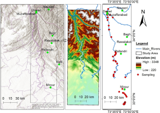
Source: OriginPro 9.1 b Application of Ward’s Linkage and Euclidean Distance method to represent water quality variables using a hierarchical clustering dendrogram model. Source: OriginPro 9.1
A comprehensive review of water quality indices (WQIs): history, models, attempts and perspectives

Water quality assessment of lake water: a review

Surface water quality analysis using multivariate statistical techniques: a case study of Fars Province rivers, Iran
Data availability.
The data supporting this study's findings can be obtained from the corresponding author upon reasonable request.
Code availability
Not applicable.
Abbas, S., & Kousar, S. (2021). Spatial analysis of drought severity and magnitude using the standardized precipitation index and streamflow drought index over the Upper Indus Basin, Pakistan. Environment, Development and Sustainability, 23 , 15314–15340.
Article Google Scholar
Alaez, M. C. F., Alaez, M. F., & Calabuig, E. L. (1988). Variations spatio-temporelle de la composition physico-chimique de la rivière Bernesga (León, Espagne). Annales De Limnologie, 24 (3), 285–291. https://doi.org/10.1051/limn/1988025
Ali, W., & Muhammad, S. (2022). Spatial distribution of contaminants and water quality assessment using an indexical approach, Astore River basin, Western Himalayas. Northern Pakistan. Geocarto International, 37 (26), 14005–14026.
APHA, A. E. G., AWWA, A. D. E., & WEF, L. S. C. (1995). Standard Methods for the Examination of Water and Wastewater . Washington D. C.: American Public Health Association.
Google Scholar
APHA. (2005). Standard Methods of Water and Wastewater. 21st Edn. In American Public Health Association (pp. 2–61). Washington, DC.
Arnell, N. W. (1999). Climate change and global water resources. Global Environmental Change, 9 , S31–S49.
Aziz, S., & Ullah, R. (2022). Assessment and spatial distribution of quality of water of the middle stretch of the river jhelum using multivariate statistical techniques. Journal of South Asian Studies, 10 (1), 19–35. https://doi.org/10.33687/jsas.010.01.3844
Bashir, N., Saeed, R., Muhammad Afzaal, D., Ahmad, A., Muhammad, N., Iqbal, J., Khan, A., Maqbool, Y., & Hameed, S. (2020). Water quality assessment of lower Jhelum canal in Pakistan by using geographic information system (GIS). Groundwater for Sustainable Development, 10 , 100357. https://doi.org/10.1016/j.gsd.2020.100357
Berhanu, M., Suryabhagavan, K. V., & Korme, T. (2023). Wetland mapping and evaluating the impacts on hydrology, using geospatial techniques: a case of Geba Watershed, Southwest Ethiopia. Geology, Ecology, and Landscapes, 7 (4), 293–310.
Bhat, S. A., Meraj, G., Yaseen, S., & Pandit, A. K. (2014). Statistical assessment of water quality parameters for pollution source identification in sukhnag stream: an inflow stream of lake Wular (Ramsar Site), Kashmir Himalaya. Journal of Ecosystems, 2014 , 898054. https://doi.org/10.1155/2014/898054
Bhutto, A. W., Bazmi, A. A., & Zahedi, G. (2012). Greener energy: Issues and challenges for Pakistan-hydel power prospective. Renewable and Sustainable Energy Reviews, 16 (5), 2732–2746.
Brown, R. M., McLelland, N. I., Deininger, R. A., & O'Connor, M. F. (1972). A water quality index - crashing the psychological barrier, Indicators of Environmental Quality. In Proceedings of a symposium held during the AAAS meeting in Philadelphia (pp. 173–182). US. Springer.
Bu, J., Liu, W., Pan, Z., & Ling, K. (2020). Comparative study of hydrochemical classification based on different hierarchical cluster analysis methods. International Journal of Environmental Research and Public Health, 17 (24), 9515.
Article CAS Google Scholar
de Andrade Costa, D., Soares de Azevedo, J. P., & dos Santos, M. A. (2020). Water quality assessment based on multivariate statistics and water quality index of a strategic river in the Brazilian Atlantic Forest. Scientific Reports . https://doi.org/10.1038/s41598-020-78563-0
Din, I. U., Muhammad, S., Rehman, I., & ur, & Tokatli, C. (2023). Spatial distribution of potentially toxic elements contaminations and risk indices of water and sediments in the Darband and Samana streams. Pakistan. Environmental Monitoring and Assessment, 195 (11), 1343.
Doneen, L. D. (1964). Notes on water quality in agriculture . University of California, Davis.
El-Rawy, M., Fathi, H., Abdalla, F., Alshehri, F., & Eldeeb, H. (2023). An integrated principal component and hierarchical cluster analysis approach for groundwater quality assessment in Jazan. Saudi Arabia. Water, 15 (8), 1466.
CAS Google Scholar
Gibbs, R. J. (1970). Mechanisms controlling world water chemistry. Science, 170 (3962), 1088–1090.
Haq, A. U., & Muhammad, S. (2023). Spatial distribution of drinking and irrigation water quality indices of Ghizer River Basin, northern Pakistan. Environmental Science and Pollution Research, 30 (8), 20020–20030.
Haq, A. U., Muhammad, S., & Tokatli, C. (2023). Spatial distribution of the contamination and risk assessment of potentially harmful elements in the Ghizer River Basin, northern Pakistan. Journal of Water and Climate Change, 14 (7), 2309–2322.
Hem, J. D. (1970). Study and interpretation of the chemical characteristics of natural water (Issue 1473). US Government Printing Office.
Ismail, E., Abdelhalim, A., & Abou Heleika, M. (2021). Hydrochemical characteristics and quality assessment of groundwater aquifers northwest of Assiut district Egypt. Journal of African Earth Sciences, 181 , 104260.
Jalal, F. A. (2021). Sustainable water supply in Pakistan: Mounting challenges and a possible source of inter-state conflicts . www.handy-signatur.at
Ji, Z.-G. (2017). Hydrodynamics and water quality: Modeling rivers, lakes, and estuaries . John Wiley & Sons.
Book Google Scholar
Khan, M. U., Malik, R. N., & Muhammad, S. (2013). Human health risk from heavy metal via food crops consumption with wastewater irrigation practices in Pakistan. Chemosphere, 93 (10), 2230–2238.
Kelley, W. P. (1963). Use of saline irrigation water. Soil science , 95 (6), 385–391.
Kumar, M., Singh, R. B., Singh, A., Pravesh, R., Majid, S. I., & Tiwari, A. (2023). Introduction of Geographic Information System. In Geographic Information Systems in Urban Planning and Management (pp. 3–24). Springer.
Kumari, M., & Rai, S. C. (2020). Hydrogeochemical evaluation of groundwater quality for drinking and irrigation purposes using water quality index in semi arid region of India. Journal of the Geological Society of India, 95 , 159–168.
Liang, Y. Q., Yong, E. L., Annammala, K. V., Bidin, K., Nainar, A., Mazilamani, L. S., & Mohamad, N. A. (2023). A comparative review on Malaysia’s water quality index model with international water quality index models for surface water quality classification. IOP Conference Series: Earth and Environmental Science, 1143 (1), 012006.
Liu, Z., Jiayi, X., Liu, M., Yin, Z., Liu, X., Yin, L., & Zheng, W. (2023). Remote sensing and geostatistics in urban water-resource monitoring: A review. Marine and Freshwater Research, 74 (10), 747–765. https://doi.org/10.1071/MF22167
Mahmood, R., & Jia, S. (2016). Assessment of impacts of climate change on the water resources of the transboundary Jhelum River basin of Pakistan and India. Water, 8 (6), 246.
Marijic, J., Li, Q., Song, M., Nishimaru, K., Stefani, E., & Toro, L. (2001). Decreased expression of voltage-and Ca2+-activated K+ channels in coronary smooth muscle during aging. Circulation Research, 88 (2), 210–216.
Mehmood, M. A., Shafiq-ur-Rehman, A. R., & Ganie, S. A. (2017). Spatio-temporal changes in water quality of Jhelum River, Kashmir Himalaya. International Journal of Environmental Bioenergy, 12 (1), 1–29.
Mir, R. A., & Jeelani, G. (2015). Hydrogeochemical assessment of river Jhelum and its tributaries for domestic and irrigation purposes, Kashmir valley India. Current Science, 109 , 311–322.
Muhammad, S., Shah, M. T., & Khan, S. (2010). Arsenic health risk assessment in drinking water and source apportionment using multivariate statistical techniques in Kohistan region, northern Pakistan. Food and Chemical Toxicology, 48 (10), 2855–2864.
Naimaee, R., Kiani, A., Jarahizadeh, S., Asadollah, H. S., & S. B., Melgarejo, P., & Jodar-Abellan, A. (2024). Long-Term Water Quality Monitoring: Using Satellite Images for Temporal and Spatial Monitoring of Thermal Pollution in Water Resources. Sustainability, 16 (2), 646.
Organization, W. H. (2017). Progress on drinking water, sanitation and hygiene: 2017 update and SDG baselines.
Patel, P. S., Pandya, D. M., & Shah, M. (2023). A holistic review on the assessment of groundwater quality using multivariate statistical techniques. Environmental Science and Pollution Research, 30 (36), 85046–85070.
Perveen, S., & Amar-Ul-Haque. (2023). Drinking water quality monitoring, assessment and management in Pakistan: A review. In Heliyon (Vol. 9, Issue 3). Elsevier Ltd. https://doi.org/10.1016/j.heliyon.2023.e13872
Radouane, E. M., Chahlaoui, A., Maliki, A., & Boudellah, A. (2023). Assessment and modeling of groundwater quality by using water quality index (WQI) and GIS technique in meknes aquifer (Morocco). Geology, Ecology, and Landscapes, 7 (2), 126–138.
Raju, N. J. (2007). Hydrogeochemical parameters for assessment of groundwater quality in the upper Gunjanaeru River basin, Cuddapah District, Andhra Pradesh, South India. Environmental Geology, 52 , 1067–1074.
Rather, M. A., Dar, B. A., Sofi, S. N., Bhat, B. A., & Qurishi, M. A. (2016). Foeniculum vulgare: A comprehensive review of its traditional use, phytochemistry, pharmacology, and safety. Arabian Journal of Chemistry, 9 , S1574–S1583. https://doi.org/10.1016/J.ARABJC.2012.04.011
Reljić, M., Romić, M., Romić, D., Gilja, G., Mornar, V., Ondrasek, G., Bubalo Kovačić, M., & Zovko, M. (2023). Advanced continuous monitoring system—tools for water resource management and decision support system in salt affected delta. Agriculture, 13 (2), 369.
Richards, L. (1954). Diagnosis and improvement of saline and alkali soils. In Handbook No. 60. Washington, DC: US Department of Agriculture.
Sabale, R., Venkatesh, B., & Jose, M. (2023). Sustainable water resource management through conjunctive use of groundwater and surface water: A review. Innovative Infrastructure Solutions, 8 (1), 17.
Sarath Prasanth, S. V., Magesh, N. S., Jitheshlal, K. V., Chandrasekar, N., & Gangadhar, K. (2012). Evaluation of groundwater quality and its suitability for drinking and agricultural use in the coastal stretch of Alappuzha District, Kerala, India. Applied Water Science, 2 , 165–175.
Schreiber, S. G., Schreiber, S., Tanna, R. N., Roberts, D. R., & Arciszewski, T. J. (2022). Statistical tools for water quality assessment and monitoring in river ecosystems – a scoping review and recommendations for data analysis. Water Quality Research Journal, 57 (1), 40–57. https://doi.org/10.2166/wqrj.2022.028
Shah, T. (2014). Groundwater governance and irrigated agriculture . Global Water Partnership (GWP) Stockholm.
Stanly, R., Yasala, S., Oliver, D. H., Nair, N. C., Emperumal, K., & Subash, A. (2021). Hydrochemical appraisal of groundwater quality for drinking and irrigation: A case study in parts of southwest coast of Tamil Nadu, India. Applied Water Science, 11 , 1–20.
Syeed, M. M., Hossain, M. S., Karim, M. R., Uddin, M. F., Hasan, M., & Khan, R. H. (2023). Surface water quality profiling using the water quality index, pollution index and statistical methods: A critical review. Environmental and Sustainability Indicators, 18 , 100247.
Tariq, A., & Mushtaq, A. (2023). Untreated wastewater reasons and causes: A review of most affected areas and cities. Int. J. Chem. Biochem. Sci, 23 , 121–143.
Tian, X., Wang, H., Liang, D., Zeng, Y., Shen, Y., Yan, Y., & Li, S. (2024). Water quality’s responses to water energy variability of the Yangtze river. Water Science & Technology, 89 (3), 635–652.
Tokatlı, C., Abu Reza, M., Islam, T., & Muhammad, S. (2024). Temporal variation of water quality parameters in the lacustrine of the Thrace Region, Northwest Türkiye. Environmental Science and Pollution Research, 31 (8), 11832–11841. https://doi.org/10.1007/s11356-024-31912-2
Uddin, M. G., Nash, S., Diganta, M. T. M., Rahman, A., & Olbert, A. I. (2023). A comparison of geocomputational models for validating geospatial distribution of water quality index. In Computational Statistical Methodologies and Modeling for Artificial Intelligence (pp. 243–276). CRC Press.
Unigwe, C. O., & Egbueri, J. C. (2023). Drinking water quality assessment based on statistical analysis and three water quality indices (MWQI, IWQI and EWQI): A case study. Environment, Development and Sustainability, 25 (1), 686–707.
US Salinity Laboratory Staff. (1954). Diagnosis and improvement of saline and alkali soils. US Department of Agricultural soils. US Department of Agricultural Hand Book 60. Washington
Wali, S. U., Alias, N. B., Bin Harun, S., Umar, K. J., Abor, I. G., Abba, A., & Buba, A. (2023). Application of principal component analysis in the context of multivariate statistics and its use for hydrogeochemical analysis. Environmental Engineering & Management Journal (EEMJ), 22 (2), 321.
Wilcox LV (1955) Classification and use of irrigation water US Department of Agri Circ 696. Washington DC.
Wu, J., Cheng, S. P., He, L. Y., Wang, Y. C., Yue, Y., Zeng, H., & Xu, N. (2023). Assessing water quality in the Pearl River for the last decade based on clustering: Characteristic, evolution and policy implications. Water Research, 244 , 120492.
Xiao, J., Gao, D., Zhang, H., Shi, H., Chen, Q., Li, H., Ren, X., & Chen, Q. (2023). Water quality assessment and pollution source apportionment using multivariate statistical techniques: A case study of the Laixi River Basin. China. Environmental Monitoring and Assessment, 195 (2), 287.
Yang, C. Y., Chang, C. C., Tsai, S. S., & Chiu, H. F. (2006). Calcium and magnesium in drinking water and risk of death from acute myocardial infarction in Taiwan. Environmental Research, 101 (3), 407–411.
Yang, D., Yang, Y., & Xia, J. (2021). Hydrological cycle and water resources in a changing world: A review. Geography and Sustainability, 2 (2), 115–122. https://doi.org/10.1016/j.geosus.2021.05.003
Zhang, Z., Shi, M., & Yang, H. (2012). Understanding Beijing’s water challenge: A decomposition analysis of changes in Beijing’s water footprint between 1997 and 2007. Environmental Science & Technology . https://doi.org/10.1021/es302576u
Zhang, H., Zhou, X., Lv, X., Xu, X., Weng, Q., & Lei, K. (2023). Exploration of the factors that influence total phosphorus in surface water and an evaluation of surface water vulnerability based on an advanced algorithm and traditional index method. Journal of Environmental Management, 342 , 118155.
Download references
Acknowledgements
The authors acknowledge the instrumental role played by the National Centre of Excellence in Geology Labs at the University of Peshawar and United Arab Emirates University in advancing scientific enquiry and fostering an environment conducive to academic excellence. Their support was integral to the success of this study.
This work was supported by the National Centre of Excellence in Geology labs at the University of Peshawar and the United Arab Emirates University. Isotope Fingerprinting of Emirates Waters, 12S158, 12S158, King Saud University, Riyadh, Saudi Arabia, RSPD2024R666, RSPD2024R666, RSPD2024R666.
Author information
Authors and affiliations.
Department of Geosciences, College of Science, United Arab Emirates University, P.O. Box 15551, Al Ain, United Arab Emirates
Tofeeq Ahmad & Alaa Ahmed
National Water and Energy Center, United Arab Emirates University, P.O. Box 15551, Al Ain, United Arab Emirates
Department of Earth Sciences, The University of Haripur, Haripur, 22620, Pakistan
Tofeeq Ahmad, Muhammad Umar & Muhammad Usman Azhar
National Centre of Excellence in Geology, University of Peshawar, Peshawar, 25130, Pakistan
Said Muhammad
Department of Chemistry, College of Science, King Saud University, 11451, Riyadh, Saudi Arabia
Ashfaq Ahmed
Department of River Ecology, Helmholtz Centre for Environmental Research-UFZ, Brückstra.3a, 39114, Magdeburg, Germany
Rizwan Ullah
You can also search for this author in PubMed Google Scholar
Contributions
Tofeeq Ahmad: Methodology–Field Investigation & Data Collection, Analysis & Interpretation, Writing–original draft; Said Muhammad: Conceptualisation, Visualisation, Supervision, Resources, Comprehensive Review & Editing; Muhammad Umar & Muhammad Usman Azhar: Co-Supervision, Fieldwork, Data Analysis; Alaa Ahmed: Software, Validation, Intellectual contributions to text/revisions; Ashfaq Ahmad: Data curation, funding, and revision. Rizwan Ullah: Data curation and revision.
Corresponding author
Correspondence to Alaa Ahmed .
Ethics declarations
Conflict of interest.
The authors declare no competing interests.
Ethical approval
Consent to participate.
All authors have reviewed and approved the final manuscript.
Consent for publication
All authors have approved for this publication.
Additional information
Publisher's note.
Springer Nature remains neutral with regard to jurisdictional claims in published maps and institutional affiliations.
Rights and permissions
Springer Nature or its licensor (e.g. a society or other partner) holds exclusive rights to this article under a publishing agreement with the author(s) or other rightsholder(s); author self-archiving of the accepted manuscript version of this article is solely governed by the terms of such publishing agreement and applicable law.
Reprints and permissions
About this article
Ahmad, T., Muhammad, S., Umar, M. et al. Spatial distribution of physicochemical parameters and drinking and irrigation water quality indices in the Jhelum River, Pakistan. Environ Geochem Health 46 , 263 (2024). https://doi.org/10.1007/s10653-024-02026-y
Download citation
Received : 30 January 2024
Accepted : 05 May 2024
Published : 01 July 2024
DOI : https://doi.org/10.1007/s10653-024-02026-y
Share this article
Anyone you share the following link with will be able to read this content:
Sorry, a shareable link is not currently available for this article.
Provided by the Springer Nature SharedIt content-sharing initiative
- Sustainable water management
- Jhelum River basin
- Azad Jammu and Kashmir
- Northern Punjab
- Geospatial distribution
- Statistical analysis
- Find a journal
- Publish with us
- Track your research
COMMENTS
This study was designed to evaluate a broad spectrum of water-quality constituents of natural water sources and household drinking water used by residents of rural communities in Limpopo Province. We also aimed to determine how water sources and collection practices change between dry and wet seasons within a one-year sampling period.
The future of deep learning in water quality. As DL becomes increasingly applied, tested and improved in old and new regimes, DL will probably become increasingly trustworthy for predicting future ...
This study builds on a growing body of evidence showing access to plumbing, water quality, and basic sanitation are lacking for a disturbingly large number of US residents by providing a ...
ogical quality of those waters. These adverse impacts include the nutrient enrichment of waters, als. known as 'eutrophication'.The damage costs of freshwater eutrophication in England and Wales have been estimated in the scientific literature at $105-160 million per year, with the policy response costs amounting to a furth.
This section describes the many benefits of water reuse projects and links users to case studies that provide project descriptions, information on policy considerations and financial and contractual information. ... Improved Water Quality. Pollution can degrade water quality and make surface waters too dirty for recreational, drinking, or ...
A case study was carried out to know the applicability of GIS tool for determining the quality of supply water. Water samples from 21 houses at different locations of Delhi were collected. Sample analysis was done for physicochemical parameters viz., pH, EC, TDS, Total Hardness, Total Alkalinity, Chloride, Fluoride, and Nitrate.
Summary of Conservation Case Studies. water rates, a public education program, a high-efficiency plumbing program, landscaping programs, and large-use programs. drawdown so that the level of water demand should stay constant until 2005. Peak demand is down 14% from 1990.
There is a general deterioration of river water quality under droughts and heatwaves (68% of compiled case studies), rainstorms and floods (51%) and under long-term climate change (56%), but in ...
The program has overcome challenges facing many of the nation's water quality trading programs to not only gain consensus on the frameworks needed to authorize trading, but also provide a broad range of ecosystem services. This paper compares the Tualatin case study with some of the commonly cited factors of successful trading programs.
A Physical Perspective of Recurrent Water Quality Degradation: A Case Study in the Jiangsu Coastal Waters, China. ... Our study interprets the vulnerability of the JCWs to pollutant enrichment from a physical perspective and finds the flushing efficiency to be a good indicator of eutrophication, providing references for environmental managers ...
Practical Considerations for the Incorporation of Biomass Fermentation into Enhanced Biological Phosphorus Removal. Case Study. 09/21/2023. 09/21/2023.
Selecting parameters. Based on a review of 30 existing WQIs, the parameters selected to calculate WQIs were divided into three types: fixed, open, and mixed systems [].The most of those WQIs have used a fixed set of parameters that is commonly called "basic" as the selected parameters are the most significant ones for water quality evaluation in the study site or region [1,2,12-18].
Former researchers have shown a correlation between the low water quality and the diabetes (El Madani fatima - zahra, 2019), as well as Oto rhino laryngological disorders and allergic diseases' appearance (Anass, 2019). 4. Conclusion. This study examines the surface water quality of the Oued Fez catchment basins.
Part of the 1983 Water Quality Assurance Act requires Florida DER to "establish a ground water quality monitoring network designed to detect and predict contamination of the State's ground water resources" via collaborative efforts with other state and federal agencies. The three basic goals of the ground water quality monitoring program are to:
1. Introduction. The water quality index (WQI) can express the water quality status in a single term. The application of WQI makes the general public more aware of the state of the surface water around them [24, 28].The Citarum River plays a key role in the life of the community and ecosystem around it, and thus accurately determining its WQI daily should help the community readily understand ...
By this study, we compare and contrast the extent to which current state-of-science technology for PWS water quality characterization (Case Study 1) and advanced technologies, HRMS-based wide ...
Principal component analysis and factor analysis showed that two factors, the degree of mineralization and agricultural runoff, and flood entrainment, explained 82.50% of the total variance. The case study demonstrates that this method is useful for evaluating and interpreting large, complex water-quality data sets.
This study presents an initial analysis of water quality input-output data necessary for black-box modeling performed using the EPANET-MATLAB toolkit with respect to an existing WDS network, Bogotá, Colombia. The methodology is based on (1) analysis of model input and output variables, (2) numerical simulation of network water quality in the ...
It is recommended to study the water quality in detail between km 67 to 73 and from km 95 to km 128 as the WQI is unfit in this region and needs more investigations in this region. ... Groundwater quality investigation using water quality index and ARCGIS: case study: Western Nile Delta Aquifer, Egypt. Eighteenth International Water Technology ...
The Water Quality Guidelines includes 2 case studies that help users to understand the theoretical particulars of the Water Quality Management Framework in a real-life setting. The case studies were contributed by government organisations involved in the protection of aquatic ecosystems in freshwater and marine waters.
Price: 750 INR (Indian reprint) Original Edition, entitled " Assessment of Drinking Water Quality: A Case Study" by Syed Mustafa Hasan Razvi, Umesh C A and Nagalambika Prasad published by ...
Rivers have always been the most significant freshwater source for life, social progress, and economic development, as ancient civilisations have prospered along with them (Varol et al. 2012).Anthropogenic activities and natural processes deteriorate surface water quality and adversely affect their importance (Singh et al. 2004; Dash et al. 2020; Prasad et al. 2020).
Table 1. Water quality parameters of the Jhenai River (February-April, 2018) The highest DO content of the river w ater was observed. 5.4mg/l at St-3 in March while the lowest was 4.2 mg/l at St ...
Sustainable management of river systems is a serious concern, requiring vigilant monitoring of water contamination levels that could potentially threaten the ecological community. This study focused on the evaluation of water quality in the Jhelum River (JR), Azad Jammu and Kashmir, and northern Punjab, Pakistan. To achieve this, 60 water samples were collected from various points within the ...